NLP – Natural Language Processing
NLP is a field in machine learning with the ability of a computer to understand, analyse, manipulate, and potentially generate human language. Its goal is to build systems that can make sense of text and perform tasks like translation, grammar checking, or topic classification.
Where NLP is being used:
- Sentiment Analysis (Hater news gives us the sentiment of the user)
- Machine Translation (Google translator, translates language from one language to another).
- Spam Filter (Gmail filters spam emails separately).
- Auto-Predict (Google Search predicts user search results).
- Speech Recognition (Google WebSpeech or Vocalware).
Library for NLP:
NLTK is a popular open-source package in Python. Rather than building all tools from scratch, NLTK provides all common NLP Tasks.
Installing NLTK:
Type !pip install nltk in the Jupyter Notebook or if it doesn’t work in cmd type conda install -c conda-forge nltk. This should work in most cases.
NLP Techniques:
Natural Language Processing (NLP) has two techniques to help computers understand text.
- Syntactic analysis
- Semantic analysis
Semantic Analysis:
Semantic analysis focuses on capturing the meaning of text. First, it studies the meaning of each individual word (lexical semantics). Then, it looks at the combination of words and what they mean in context. The main sub-tasks of semantic analysis are:
- Word sense disambiguation tries to identify in which sense a word is being used in a given context.
- Relationship extraction attempts to understand how entities (places, persons, organizations, etc) relate to each other in a text.
Semantic analysis:
It focuses on identifying the meaning of language. Semantic tasks analyze the structure of sentences, word interactions, and related concepts, in an attempt to discover the meaning of words, as well as understand the topic of a text.
Following are the list of some of the main sub-tasks of both semantic and syntactic analysis:
Tokenisation:
Tokenizing separates text into units such as sentences or words. Sentence tokenization splits sentences within a text, and word tokenization splits words within a sentence. Generally, word tokens are separated by blank spaces, and sentence tokens by stops.
Here’s an example of how word tokenization simplifies text: Customer service couldn’t be better! = “customer service” “could” “not” “be” “better”.
Remove punctuation:
Punctuation can provide grammatical context to a sentence which supports our understanding. But for our vectorizer which counts the number of words and not the context, it does not add value, so we remove all special characters.
eg: How are you?->How are you
Remove stopwords:
Stopwords are common words that will likely appear in any text. They don’t tell us much about our data so we remove them.
example: “Hello, I’m having trouble logging in with my new password”, it may be useful to remove stop words like “hello”, “I”, “am”, “with”, “my”, so you’re left with the words that help you understand the topic of the ticket: “trouble”, “logging in”, “new”, “password”.
Stemming:
Stemming helps reduce a word to its stem form. It often makes sense to treat related words in the same way. It removes suffices, like “ing”, “ly”, “s”, etc. by a simple rule-based approach. It reduces the corpus of words but often the actual words get neglected.
eg: Entitling,Entitled->Entitl Stemming “trims” words, so word stems may not always be semantically correct. For example, stemming the words “consult,” “consultant,” “consulting,” and “consultants” would result in the root form “consult.”
Lemmatizing:
Lemmatizing derives the canonical form (‘lemma’) of a word. i.e the root form. It is better than stemming as it uses a dictionary-based approach i.e a morphological analysis to the root word.
Lemmatizing derives the canonical form (‘lemma’) of a word. i.e the root form. It is better than stemming as it uses a dictionary-based approach i.e a morphological analysis to the root word.
So summery is Stemming is typically faster as it simply chops off the end of the word, without understanding the context of the word. Lemmatizing is slower and more accurate as it takes an informed analysis with the context of the word in mind.
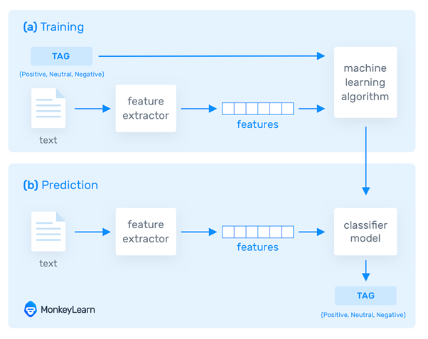
Vectorizing Data:
Vectorizing is the process of encoding text as integers i.e. numeric form to create feature vectors so that machine learning algorithms can understand our data.
Following are the vectorization technique:
Bag-Of-Words:
Bag of Words (BoW) or CountVectorizer describes the presence of words within the text data. It gives a result of 1 if present in the sentence and 0 if not present. It, therefore, creates a bag of words with a document-matrix count in each text document.
Now lets understand with the movie review example.
- Review 1: This movie is very scary and long
- Review 2: This movie is not scary and is slow
- Review 3: This movie is spooky and good
We will first build a vocabulary from all the unique words in the above three reviews. The vocabulary consists of these 11 words: ‘This’, ‘movie’, ‘is’, ‘very’, ‘scary’, ‘and’, ‘long’, ‘not’, ‘slow’, ‘spooky’, ‘good’.
We can now take each of these words and mark their occurrence in the three movie reviews above with 1s and 0s. This will give us 3 vectors for 3 reviews:
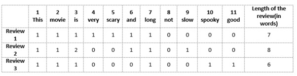
Vector of Review 1: [1 1 1 1 1 1 1 0 0 0 0]
Vector of Review 2: [1 1 2 0 0 1 1 0 1 0 0]
Vector of Review 3: [1 1 1 0 0 0 1 0 0 1 1]
And that’s the core idea behind a Bag of Words (BoW) model.
In the above example, we can have vectors of length 11. However, we start facing issues when we come across new sentences:
- If the new sentences contain new words, then our vocabulary size would increase and thereby, the length of the vectors would increase too.
- Additionally, the vectors would also contain many 0s, thereby resulting in a sparse matrix (which is what we would like to avoid)
- We are retaining no information on the grammar of the sentences nor on the ordering of the words in the text.
TF-IDF(Term frequency-inverse document frequency)
tf-idf stands for Term frequency-inverse document frequency. The tf-idf weight is a weight often used in information retrieval and text mining. Variations of the tf-idf weighting scheme are often used by search engines in scoring and ranking a document’s relevance given a query. This weight is a statistical measure used to evaluate how important a word is to a document in a collection or corpus. The importance increases proportionally to the number of times a word appears in the document but is offset by the frequency of the word in the corpus (data-set).
“Term frequency–inverse document frequency, is a numerical statistic that is intended to reflect how important a word is to a document in a collection or corpus”
Let’s recall the three types of movie reviews we saw earlier:
- Review 1: This movie is very scary and long
- Review 2: This movie is not scary and is slow
- Review 3: This movie is spooky and good
Step 1: Computing the Term Frequency(tf)
Let’s first understand Term Frequent (TF). It is a measure of how frequently a term, t, appears in a document, d:
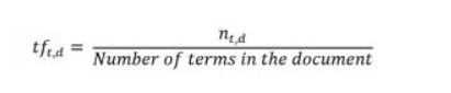
Here, in the numerator, n is the number of times the term “t” appears in the document “d”. Thus, each document and term would have its own TF value.
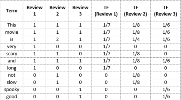
We will again use the same vocabulary we had built in the Bag-of-Words model to show how to calculate the TF for Review #2:
Review 2: This movie is not scary and is slow
Here,
- Vocabulary: ‘This’, ‘movie’, ‘is’, ‘very’, ‘scary’, ‘and’, ‘long’, ‘not’, ‘slow’, ‘spooky’, ‘good’
- Number of words in Review 2 = 8
- TF for the word ‘this’ = (number of times ‘this’ appears in review 2)/(number of terms in review 2) = 1/8
Similarly,
- TF(‘movie’) = 1/8
- TF(‘is’) = 2/8 = 1/4
- TF(‘very’) = 0/8 = 0
- TF(‘scary’) = 1/8
- TF(‘and’) = 1/8
- TF(‘long’) = 0/8 = 0
- TF(‘not’) = 1/8
- TF(‘slow’) = 1/8
- TF( ‘spooky’) = 0/8 = 0
- TF(‘good’) = 0/8 = 0
We can calculate the term frequencies for all the terms and all the reviews in this manner:
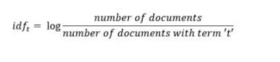
Step 2: Compute the Inverse Document Frequency – idf
The inverse document frequency of the word across a set of documents. This means, how common or rare a word is in the entire document set. It typically measures how important a term is. The main purpose of doing a search is to find out relevant documents matching the query. Since tf considers all terms equally important, thus, we can’t only use term frequencies to calculate the weight of a term in the document. However, it is known that certain terms, such as “is”, “of”, and “that”, may appear a lot of times but have little importance. Thus we need to weigh down the frequent terms while scaling up the rare ones. Logarithms helps us to solve this problem.
We can calculate the IDF values for the all the words in Review 2:
IDF(‘this’) = log(number of documents/number of documents containing the word ‘this’) = log(3/3) = log(1) = 0
Similarly,
- IDF(‘movie’, ) = log(3/3) = 0
- IDF(‘is’) = log(3/3) = 0
- IDF(‘not’) = log(3/1) = log(3) = 0.48
- IDF(‘scary’) = log(3/2) = 0.18
- IDF(‘and’) = log(3/3) = 0
- IDF(‘slow’) = log(3/1) = 0.48
We can calculate the IDF values for each word like this. Thus, the IDF values for the entire vocabulary would be:
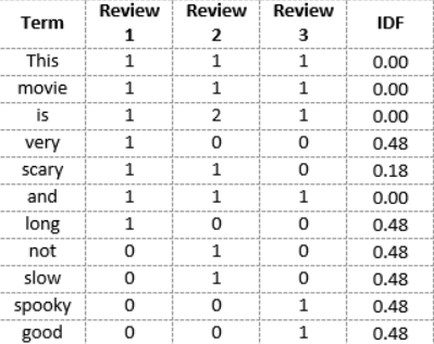
Hence, we see that words like “is”, “this”, “and”, etc., are reduced to 0 and have little importance; while words like “scary”, “long”, “good”, etc. are words with more importance and thus have a higher value.
We can now compute the TF-IDF score for each word in the corpus. Words with a higher score are more important, and those with a lower score are less important:
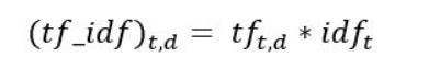
We can now calculate the TF-IDF score for every word in Review 2:
TF-IDF(‘this’, Review 2) = TF(‘this’, Review 2) * IDF(‘this’) = 1/8 * 0 = 0
Similarly,
- TF-IDF(‘movie’, Review 2) = 1/8 * 0 = 0
- TF-IDF(‘is’, Review 2) = 1/4 * 0 = 0
- TF-IDF(‘not’, Review 2) = 1/8 * 0.48 = 0.06
- TF-IDF(‘scary’, Review 2) = 1/8 * 0.18 = 0.023
- TF-IDF(‘and’, Review 2) = 1/8 * 0 = 0
- TF-IDF(‘slow’, Review 2) = 1/8 * 0.48 = 0.06
Similarly, we can calculate the TF-IDF scores for all the words with respect to all the reviews:
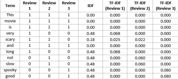
We have now obtained the TF-IDF scores for our vocabulary. TF-IDF also gives larger values for less frequent words and is high when both IDF and TF values are high i.e the word is rare in all the documents combined but frequent in a single document.
Note-
While both Bag-of-Words and TF-IDF have been popular in their own regard, there still remained a void where understanding the context of words was concerned. Detecting the similarity between the words ‘spooky’ and ‘scary’, or translating our given documents into another language, requires a lot more information on the documents.
N-Grams:
N-grams are simply all combinations of adjacent words or letters of length n that we can find in our source text. Ngrams with n=1 are called unigrams. Similarly, bigrams (n=2), trigrams (n=3) and so on can also be used. Unigrams usually don’t contain much information as compared to bigrams and trigrams. The basic principle behind n-grams is that they capture the letter or word is likely to follow the given word. The longer the n-gram (higher n), the more context you have to work with.
In Next chapter we will implement NLP concept with the help of python.