Category Machine Learning

Data Science – An Introduction

What is Data science?

It is a study that deals with the identification and extraction of meaningful information from data sources with the help of various scientific methods and algorithms. This helps in better decision making, promotional offers and predictive analytics for any business or organization.

What are the skills required to be a Data scientist?

  • Programing Skill
    • Python
    • R
    • Database Query Languages.
  • Statistics and Probability
  • BI Tools – Tableau, Power BI, Qlik Sense
  • Business Domain Knowledge

Data Science Life Cycle:


Data Scientist VS  Data Analyst VS  Data Engineer

 Data Analyst:

It is an entry-level job for those professionals who are interested in getting into a data-related job. Organisation expect from Data Analyst to understand data handling, modeling and reporting techniques along with a strong understanding of the business. A Data analyst required a good knowledge of visualization tools and database. There are two most popular and common tools used by the data analysts are SQL and Microsoft Excel.

It is necessary for the data analyst to have good presentation skills. This helps them to communicate the end results with the team and help them to reach proper solutions.

Data Engineer:

A Data Engineer specializes in preparing data for analytical usage. They have good idea about Data pipelining with performance optimization. A Data Engineer required strong technical background with the ability to create and integrate APIs. Data Engineering also involves the development of platforms and architectures for data processing.

So what skills required being a Data Engineer?

  • Data Warehousing & ETL
  • Advanced programming knowledge
  • Machine learning concept knowledge
  • In-depth knowledge of SQL/ database
  • Hadoop-based Analytics
 
Data Scientist:

A data scientist is a person who applies their knowledge in statistics and building machine learning models to make predictions to answer the key business questions. They use to deal with big messy data set and a big data wranglers. They apply their math, programing and statistics skills on the data set to clean and organize.

Once data is in clean form then Data scientist apply machine learning algorithm to find hidden insights in the data and draw a meaningful summary out of that.

Skill set for a data scientist:-

  • In depth programing knowledge of SAS/R/Python.
  • Statistics and Mathematics concepts.
  • Machine learning algorithm.
  • Python library such as Pandas, numpy, scypi, Matplotlib, Seaborn, StatsModels.

Machine Learning – Introduction

What is machine learning?

Machine learning is a field of computer science which gives computer to learn from example through self-improvement and without being explicitly coded by programmer. In simple words, ML is a type of artificial intelligence that extracts patterns out of raw data by using an algorithm or method.  It is the most exciting technology in recent years.

ML is used in various tasks like fraud detection, predictive maintenance, portfolio optimization, automate task, clustering, sentiment analysis, image recognition, recommendation system and many more.

Prerequisites for Machine learning:

Reader should know basic python, python library like NumPy, Scikit-learn, Scipy, Matplotlib and seaborn. If these topics are new for you then we highly recommend you please go through Python for Data Science Tutorial.

Why Machine Learning?

Let’s understand it with an example, Think of a day when the sky is full of dark clouds and thunderstorms. The 1st thing that comes to your mind is, it’s going to rain today.

How did you know that it’s going to rain?

You know it because, in your life, whenever you have seen the sky behaving the same then it has rained, that’s what Machine Learning is all about.  

A machine is train to be learn from past experiences (data feed in) with respect to some class of tasks and it is performance in a given task improves with the experience.

Any technology user today has benefitted from machine learning. Facial recognition technology allows social media platforms to help users tag and share photos of friends. Optical character recognition (OCR) technology converts images of text into movable type. Recommendation engines, powered by machine learning, suggest what movies or television shows to watch next based on user preferences. Self-driving cars that rely on machine learning to navigate may soon be available to consumers. Risk analysis  for banking and finance industry. These all types of work is happening through machine learning.

Machine Learning Lifecycle:

Data Science process

What does it hold for the future?

Remember the robot helpers you saw in I, Robot? Imagine those in our day-to-day lives. Helping clean up our homes and generally making life even easier.

Traffic annoying you? How about you relaxed in the air conditioning of your car, and it took care of taking you to your destination? On its own?

Or how about as soon as you entered your doctor’s office, they have access to all your relevant medical details. Enabling them to provide you with a more personalized diagnosis?

Below image are few among hundreds of ways it makes our lives easier.

Future of machine learning

Types of Machine Learning

There are several Machine Learning algorithm and techniques which is used to build models for solving real-life problems by using data.

Now let’s discuss each type in details.

Supervised Learning:

Supervised learning technique is use when data set is structured. Structured dataset is one which has both input and output parameters. It is called supervised learning because we have a dataset which acts as a teacher and its role is to train the model or the machine. Once the model gets trained it can start making a prediction or decision when new data is given to it.

Supervised learning is the one where you have input variables (x) and an output variable (Y) and you use an algorithm to learn the mapping function from the input to the output.

Y = f(X)

The goal is to approximate the mapping function so well that whenever you get  new input data (x), the machine can easily predict the output variables (Y) for that data.

Supervised Learning Process

Unsupervised Learning:

Unsupervised learning is where we only have input data (X) and no corresponding output variables i.e Y.

The unsupervised model learns through observation and finds structures in the data. Once the model is given a dataset, it automatically finds patterns and relationships in the dataset by creating clusters in it. Unsupervised learning is used for raw datasets. Its main task is to convert raw data to structured data.

Unsupervised learning process

Now let’s understand both type of learning in details with example.

Suppose you had a basket and it is filled with some different kinds of fruits, your task is to arrange them as groups. For understanding let me clear the names of the fruits in our basket. We have four types of fruits. They are: apple, banana, grape and cherry.

SUPERVISED LEARNING:

  • You already learn from your previous work about the physical characters of fruits.
  • So arranging the same type of fruits at one place is easy now.
  • Your previous work is called as training data in data mining.
  • So, you already learn the things from your train data, this is because of response variable.
  • Response variable mean just a decision variable.

You can observe response variable below (FRUIT NAME) .

NO. SIZE COLOR SHAPE FRUIT NAME
1 Big Red Rounded shape with a depression at the top Apple
2 Small Red Heart-shaped to nearly globular Cherry
3 Big Green Long curving cylinder Banana
4 Small Green Round to oval, Bunch shape Cylindrical Grape
  • Suppose you have taken an new fruit from the basket then you will see the size, color and shape of that particular fruit.
  • If size  is Big, color is Red, shape is rounded shape with a depression at the top, you will conform the fruit name as apple and you will put in apple group. Likewise for other fruits also.
  • Job of groping fruits was done and happy ending.
  • You can observe in the table that  a column was labelled as “FRUIT NAME” this is called as response variable.
  • If you learn the thing before from training data and then applying that knowledge to the test data(for new fruit), This type of learning is called as Supervised Learning.
  • Classification come under Supervised learning.

UNSUPERVISED LEARNING

  • Suppose you had a basket and it is filled with some different types fruits,your task is to arrange them as groups.
  • This time you don’t know anything about that fruits, honestly saying this is the first time you have seen them.
  • So how will you arrange them? What will you do first?
  • You will take a fruit and you will arrange them by considering physical character of that particular fruit. suppose you have considered color.
  • Then you will arrange them on considering base condition as color.
  • Then the groups will be something like this.
  • RED COLOR GROUP: apples & cherry fruits.
  • GREEN COLOR GROUP: bananas & grapes.
  • So now you will take another physical character such as size .
  • RED COLOR AND BIG SIZE: apple.
  • RED COLOR AND SMALL SIZE: cherry fruits.
  • GREEN COLOR AND BIG SIZE: bananas.
  • GREEN COLOR AND SMALL SIZE: grapes.
  • Job done happy ending.
  • Here you didn’t know learn anything before, means no train data and no response variable.
  • This type of learning is known as unsupervised learning.
  • Clustering comes under unsupervised learning.

Semi-Supervised Learning:

As per name suggestion same supervised learning is a combination of Supervise learning and unsupervised learning and uses both labelled and unlabelled data for training. We use this type of Machine Learning for classification, regression, and prediction. Examples of semi-supervised learning are face- and voice-recognition applications.

Reinforcement Learning:

It follows traditional types of data analysis where algorithm discovers data through a process of trial and error and find out what is the best outcome.

There are three main components make up reinforcement learning: the agent, the environment, and the actions. The agent is the learner or decision-maker, the environment includes everything that the agent interacts with, and the actions are what the agent does.

Reinforcement Learning Process

Following are the hierarchy of machine learning.

Principal component Analysis(PCA)-Theory

In real world scenario data analysis tasks involve complex data analysis i.e. analysis for multi-dimensional data. We analyse the data and try to find out various patterns in it.

Here dimensions represents your data point x, As the dimensions of data increases, the difficulty to visualize it and perform computations on it also increases. So, how to reduce the dimensions of a data

  • Remove the redundant dimension
  • Only keep the most important dimension

To reduce dimensions of the data we use principle component analysis. Before we deep dive in working of PCA, lets understand some key terminology, which will use further.

Variance:

It is a measure of the variability or it simply measures how spread the data set is. Mathematically, it is the average squared deviation from the mean score. We use the following formula to compute variance var(x).

Covariance: It is a measure of the extent to which corresponding elements from two sets of ordered data move in the same direction. Formula is shown above denoted by cov(x,y) as the covariance of x and y.

Here, xi is the value of x in ith dimension. x bar and y bar denote the corresponding mean values.
One way to observe the covariance is how interrelated two data sets are.

Positive, negative and zero covariance:

Positive covariance means X and Y are positively related i.e. as X increases Y also increases. Negative covariance depicts the exact opposite relation. However zero covariance means X and Y are not related.

Eigenvectors and Eigenvalues:

To better understand these concepts, let’s consider the following situation. We are provided with 2-dimensional vectors v1, v2, …, vn. Then, if we apply a linear transformation T (a 2×2 matrix) to our vectors, we will obtain new vectors, called b1, b2,…,bn.

Some of them (more specifically, as many as the number of features), though, have a very interesting property: indeed, once applied the transformation T, they change length but not direction. Those vectors are called eigenvectors, and the scalar which represents the multiple of the eigenvector is called eigenvalue

Thus, each eigenvector has a correspondent eigenvalue.

When should I use PCA:

  1. If you want to reduce the number of variables, but aren’t able to identify variables to completely remove from consideration?
  2. If you want to ensure your variables are independent from each other.
  3. To avoid overfitting your model.
  4. If you are comfortable making your independent variable less interpretable.

Background:

  • PCA is an unsupervised statistical technique used to examine the interrelations among a set of variables in order to identify the underlying structure of those variables.
  • It is also known sometimes as a general factor analysis.
  • Where regression determines a line of best fit to a data set, factor analysis determines several orthogonal lines of best fit to the data set.
  • Orthogonal means “at right angles”.
    • Actually the lines are perpendicular to each other in n-dimensional space.
  • N-dimensional Space is the variable sample space.
    • There are as many dimensions as there are variables, so in a data set with 4 variables the sample space is 4-dimensional.
  • Here we have some data plotted along two features, x and y.
  • We can add an orthogonal line. Now we can begin to understand the components!
  • Components are a linear transformation that chooses a variable system for the data set such that the greatest variance of the data set comes to lie on the first axis.
  • The second greatest variance on the second axis, and so on.
  • This process allows us to reduce the number of variables used in an analysis.
  • We can continue this analysis into higher dimensions.
  • If we use this technique on a data set with a large number of variables, we can compress the amount of explained variation to just a few components.
  • The most challenging part of PCA is interpreting the components.

For our work with Python, we’ll walk through an example of how to perform PCA with scikit learn. We usually want to standardize our data by some scale for PCA, so we’ll cover how to do this as well.

PCA Algorithm

  • Calculate the covariance matrix X of data points.
  • Calculate eigenvectors and corresponding eigenvalues.
  • Sort the eigen vectors according to their eigenvalues in decreasing order.
  • Choose first k eigenvectors and that will be the new k dimensions.
  • Transform the original n dimensional data points into k dimensions.

Advantages of PCA

  1. Removes Correlated Features: In a real world scenario, this is very common that you get thousands of features in your dataset. You cannot run your algorithm on all the features as it will reduce the performance of your algorithm and it will not be easy to visualize that many features in any kind of graph. So, you MUST reduce the number of features in your dataset. You need to find out the correlation among the features (correlated variables). Finding correlation manually in thousands of features is nearly impossible, frustrating and time-consuming. PCA does this for you efficiently.
  2. Improves Algorithm Performance: With so many features, the performance of your algorithm will drastically degrade. PCA is a very common way to speed up your Machine Learning algorithm by getting rid of correlated variables which don’t contribute in any decision making. The training time of the algorithms reduces significantly with less number of features. So, if the input dimensions are too high, then using PCA to speed up the algorithm is a reasonable choice.
  3. Improves Visualization: It is very hard to visualize and understand the data in high dimensions. PCA transforms a high dimensional data to low dimensional data (2 dimension) so that it can be visualized easily. We can use 2D Scree Plot to see which Principal Components result in high variance and have more impact as compared to other Principal Components.

Disadvantages of PCA

  1. Independent variables become less interpretable: After implementing PCA on the dataset, your original features will turn into Principal Components. Principal Components are the linear combination of your original features. Principal Components are not as readable and interpretable as original features.
  2. Data standardization is must before PCA: You must standardize your data before implementing PCA, otherwise PCA will not be able to find the optimal Principal Components. For instance, if a feature set has data expressed in units of Kilograms, Light years, or Millions, the variance scale is huge in the training set. If PCA is applied on such a feature set, the resultant loadings for features with high variance will also be large. Hence, principal components will be biased towards features with high variance, leading to false results.
  3. Information Loss: Although Principal Components try to cover maximum variance among the features in a dataset, if we don’t select the number of Principal Components with care, it may miss some information as compared to the original list of features.

Reference:

Medium

PCA with python

In this lecture we will implement PCA algorithm through Python. We will also see how to reduce features in the data set.

About Minist Data Set

The MNIST dataset (Modified National Institute of Standards and Technology database) is a large dataset of handwritten digits that is commonly used for training various image processing systems. Available on kaggle (https://www.kaggle.com/c/digit-recognizer/data)

The database is also widely used for training and testing in the field of machine learning.

  • The dataset consists of pair, “handwritten digit image” and “label”. Digit ranges from 0 to 9, meaning 10 patterns in total. handwritten digit image: This is gray scale image with size 28 x 28 pixel.
  • label : This is actual digit number this handwritten digit image represents. It is either 0 to 9.

Our Objective

In this data sets around 42000 rows and 784 columns are available, we will try to reduce features from 784, so that we will have less features and maximum information.

Let’s explore the concept through jupyter notebook.

Classification VS Regression

Before going to start working on machine learning model, we need to understand difference between classification and regression problem. Classification and Regression are two major prediction problems which are usually dealt in Data mining.

Although Classification and Regression come under the same umbrella of Supervised Machine Learning and share the common concept of using past data to make predictions, or take decisions, that’s where their similarity ends.

Regression in machine learning:

A regression problem is when the output variable is a real or continuous value, such as “salary” or “weight” or “sales”.

In machine learning, regression algorithms try to calculate the mapping function (f) from the input variables (x) to numerical or continuous output variables (y). In this case, y is a real value, which can be an integer or a floating point value. Therefore, regression prediction problems are usually quantities or sizes.

For example, when provided with a dataset about houses and you are asked to predict their prices that are a regression task because price will be a continuous output.

Common regression algorithms are: Linear regression, Support Vector Regression (SVR), and regression trees.

Note – Logistic regression, have the name “regression” in their names but they are not regression algorithms.

Classification in machine learning:

A classification problem is when the output variable is a category, such as “black” or “blue” or “disease” and “no disease”.

In classification algorithms we try to calculate the mapping function (f) from the input variables (x) to discrete or categorical output variables (y).

For example, we have a house dataset and we have to predict whether the prices for the houses “sell more or less than the recommended retail price”.  Here, the houses will be classified whether their prices fall into two discrete categories: above or below the said price.

Common classification algorithms are logistic regression, Naïve Bayes, decision trees, and K Nearest Neighbours.

So following are the main differences:

Basic for comparisonClassificationRegression
DefinitionA classification problem is when the output variable
is category such as ‘blue’
or ‘black’, disease and
no disease
A regression problem is
when the output variable is real or continuous value
such as sales, weight, salary
Involve prediction ofCategorical valueContinuous value
AlgorithmDecision tree, logistic regression, etcRegression tree (Random forest), Linear regression, etc.
Nature of the predicted dataUnorderedOrdered
Method of calculationMeasuring accuracy Measurement of root mean square error

Linear Regression-Theory

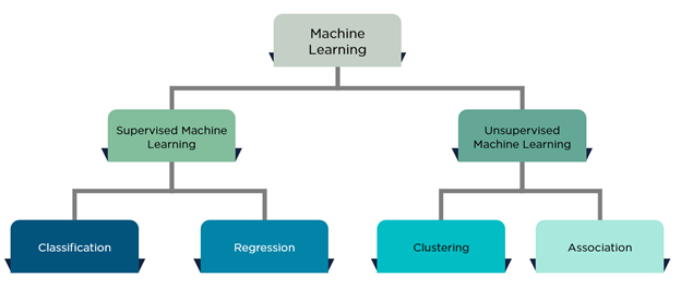
Linear regression is a supervised machine learning technique where we need to predict a continuous output, which has a constant slope.

There are two main types of linear regression:

1. Simple Regression:

Through simple linear regression we predict response using single features.

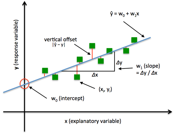
If you recall, the line equation (y = mx + c) we studied in schools. Let’s understand what these parameters say and how this equation works in linear regression.

Y = βo + β1X + ∈

Where, Y = Dependent Variable ( This is the variable which we want to predict )

            X = Independent Variable ( This is the variable which we use to make prediction )

            βo – This is the intercept term. It is the prediction value you get when X = 0

            β1 – This is the slope term. It explains the change in Y when X changes by 1 unit.

∈ – This represents the residual value, i.e. the difference between actual and predicted values.

2. Multivariable regression:

It is nothing but extension of simple linear regression. It attempts to model the relationship between two or more features and a response by fitting a linear equation to observed data.

Multi variable linear equation might look like this, where w represents the coefficients, or weights, our model will try to learn.

f(x,y,z)=w1x+w2y+w3z

Let’s understand it with example.

In a company for sales predictions, these attributes might include a company’s advertising spend on radio, TV, and newspapers.

Sales=w1Radio+w2TV+w3News

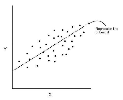
Linear Regression geometrical representation

So our goal in linear regression model is:

Find a line or plane that best fits the data points. Here best fit means minimise the sum of errors across our training data.

Types of Deliverable in linear regression:

Typically there are following questions that a business wanted to know

  1. They wanted to know their sales or profit prediction.
  2. Drivers(What drives the sales?)
    • All variable that have significant beta.
    • Which factors are detrimental /incremental?
    •  All the drivers, which one should target first?(Variable with highest absolute value)
  3. How to predict drivers?
    • To answer this question, you need calculate (beta*X )for each X variable and you need to choose the highest value and accordingly you can choose your driver after that convince business why you have chosen the particular driver.

So now the question arises how we calculate Beta values?

To calculate the beta values we will use OLS(ordinary least squared) method.

Assumptions of Linear Regression:

1. X variables (Explanatory variable) should be linearly related to Y (Response Variable):

Meaning:

If you plot a scatter plot between x variable and Y, most of the data point should be around the straight line.

How to check?

Draw the scatter plot between each x variable and y variable.

What happens if the assumption is violated?

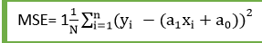
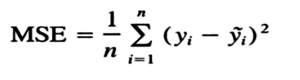
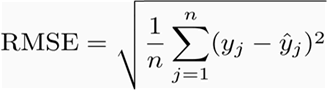
MSE(Mean Squared Error) will be high. MSE is nothing but the average of squared error occurred between the predicted values and actual values. It can be written as:

Linear Regression in Machine Learning

Where,

N=Total number of observation
Yi = Actual value
(a1xi+a0)= Predicted value.

What to do if variable is not linear?

  • Drop the variable – But in this case will loose the information.
  • Take log(x+1) of x variables. 

2.Residual or the Y variable should be normally distributed:

Meaning:

Residuals (errors) or Y, when plotted in a histogram produces a bell shaped curve.

Residuals: The distance between the actual value and predicted values is called residual. If the observed points are far from the regression line, then the residual will be high, and so cost function will high. If the scatter points are close to the regression line, then the residual will be small and hence the cost function.

How to check?

Plot a histogram of Y, when plotted histogram produces a bell- shaped curve then it follows normality.

Or we can also use  q-q plot(quantile- quantile plot) of residuals

What happens if the assumption is violated?

It means all the P values has been calculated wrongly.

What to do if assumption is violated?

In that case we need to transform our Y such a way so that it become normal. To do that we need to use log of Y.

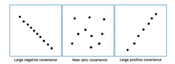
3.There should not be any relationship between X variables (i.e no multicollinearity)

Meaning:

X variable should not have any linear relationship between themselves. It’s obvious that we don’t want same information in repeat mode.

How to check?

  1. Calculate correlation between every X with every other X variable.
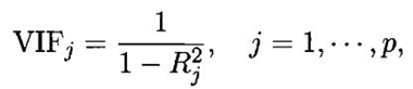
  2. Second method is to, calculate VIF(Variance influence factor)

What happens if the assumption is violated?

Your beta’s values sign will fluctuate.

What to do if assumption is violated?

Drop those X variable whose VIF is greater than 10(VIF>10)

4. The variance of error should remain constant over value of Y (Homoscedasticity/ No heteroskedasticity )

Meaning:

Spread of residuals should remain constant with values of Y.

How to check?

Draw scatter plot of residuals VS Y.

What happens if the assumption is violated?

Your P value will not accurate.

What to do if assumption is violated?

In that case we need to transform our Y such a way so that it become normal. To do that we need to use log of Y.

5. There should not be any auto-correlation between the residuals.

Meaning:

Correlation of residuals with lead residuals. Here lead residuals means next calculated residual.

How to check?

Use DW stats(Durbin Watson Stats)

            If DW stats ~ 2, then no auto correlation.

What happens if the assumption is violated?

Your P value will not accurate.

What to do if assumption is violated?

Understand the reason why it is happening?

If autocorrelation is due to Y then cannot build linear regression model.

If autocorrelation is due to X then drop that X variable.

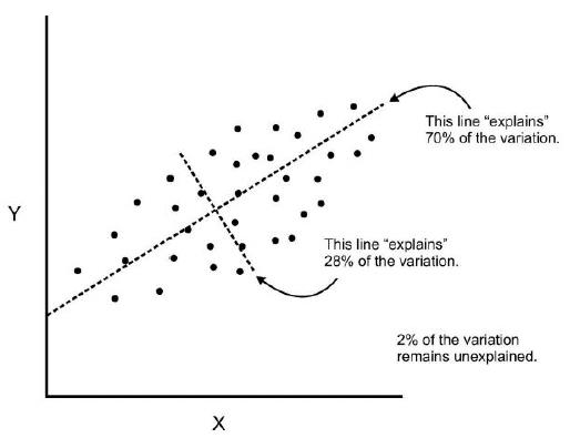
How to check Model Performance?

The Goodness of fit determines how the line of regression fits the set of observations. The process of finding the best model out of various models is called optimization. It can be achieved by below method:
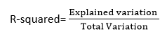
R-squared method:

  • R-squared is a statistical method that determines the goodness of fit.
  • It measures the strength of the relationship between the dependent and independent variables on a scale of 0-100%.
  • The high value of R-square determines the less difference between the predicted values and actual values and hence represents a good model.
  • It is also called a coefficient of determination, or coefficient of multiple determination for multiple regression.
  • It can be calculated from the below formula:
Linear Regression in Machine Learning

In the next lecture we will see how to implement leaner regression in python.

Linear regression with python

Company Objective:

Let’s suppose You just got some contract work with an Ecommerce company based in New York City that sells clothing online but they also have in-store style and clothing advice sessions. Customers come in to the store, have sessions/meetings with a personal stylist, then they can go home and order either on a mobile app or website for the clothes they want.

The company is trying to decide whether to focus their efforts on their mobile app experience or their website. They’ve hired you on contract to help them figure it out! Let’s get started!

Just follow the steps below to analyze the customer data (it’s fake, don’t worry I didn’t give you real credit card numbers or emails ). Click here to download

Click here to download .ipnyb notebook

Linear Regression Interview Questions and Answers

What is linear regression?

In simple terms, linear regression is a method of finding the best straight line fitting to the given data, i.e. finding the best linear relationship between the independent and dependent variables.

In technical terms, linear regression is a machine learning algorithm that finds the best linear-fit relationship on any given data, between independent and dependent variables. It is mostly done by the Sum of Squared Residuals Method.

To Know more about linear regression Click Here

What are the important assumptions of Linear regression?

Following are the assumptions

  • A linear Relationship – Firstly, there has to be a linear relationship between the dependent and the independent variables. To check this relationship, a scatter plot proves to be useful.
  • Restricted Multi-collinearity value – Secondly, there must no or very little multi-collinearity between the independent variables in the dataset. The value needs to be restricted, which depends on the domain requirement.
  • Homoscedasticity – The third is the homoscedasticity. It is one of the most important assumptions which states that the errors are equally distributed. To Know more about assumption click here

What is heteroscedasticity?

Heteroscedasticity is exactly the opposite of homoscedasticity, which means that the error terms are not equally distributed. To correct this phenomenon, usually, a log function is used.

What is the difference between R square and adjusted R square?

R square and adjusted R square values are used for model validation in case of linear regression. R square indicates the variation of all the independent variables on the dependent variable. I.e. it considers all the independent variable to explain the variation. In the case of Adjusted R squared, it considers only significant variables (P values less than 0.05) to indicate the percentage of variation in the model. To know more about R square and adjusted R square click here.

Can we use linear regression for time series analysis?

One can use linear regression for time series analysis, but the results are not promising. So, it is generally not advisable to do so. The reasons behind this are.

  1. Time series data is mostly used for the prediction of the future, but linear regression seldom gives good results for future prediction as it is not meant for extrapolation.
  2. Mostly, time series data have a pattern, such as during peak hours, festive seasons, etc., which would most likely be treated as outliers in the linear regression analysis

What is VIF? How do you calculate it?

Variance Inflation Factor (VIF) is used to check the presence of multicollinearity in a data set. It is calculated as

Here, VIFj  is the value of VIF for the jth variable, Rj2 is the R2 value of the model when that variable is regressed against all the other independent variables.

If the value of VIF is high for a variable, it implies that the R2  value of the corresponding model is high, i.e. other independent variables are able to explain that variable. In simple terms, the variable is linearly dependent on some other variables.

How to find RMSE and MSE?

RMSE and MSE are the two of the most common measures of accuracy for a linear regression.

RMSE indicates the Root mean square error, which indicated by the formula:

RMSE-Linear Regression

Where MSE indicates the Mean square error represented by the formula:

MSE-Linear Regression

How to interpret a Q-Q plot in a Linear regression model?

A Q-Q plot is used to check the normality of errors. In the above chart mentioned, Majority of the data follows a normal distribution with tails curled. This shows that the errors are mostly normally distributed but some observations may be due to significantly higher/lower values are affecting the normality of errors.

What is the significance of an F-test in a linear model?

The use of F-test is to test the goodness of the model. When the model is re-iterated to improve the accuracy with changes, the F-test values prove to be useful in terms of understanding the effect of overall regression.

What are the disadvantages of the linear model?

Linear regression is sensitive to outliers which may affect the result.

– Over-fitting

– Under-fitting

You run your regression on different subsets of your data, and in each subset, the beta value for a certain variable varies wildly. What could be the issue here?

This case implies that the dataset is heterogeneous. So, to overcome this problem, the dataset should be clustered into different subsets, and then separate models should be built for each cluster. Another way to deal with this problem is to use non-parametric models, such as decision trees, which can deal with heterogeneous data quite efficiently.

Which graphs are suggested to be observed before model fitting?

Before fitting the model, one must be well aware of the data, such as what the trends, distribution, skewness, etc. in the variables are. Graphs such as histograms, box plots, and dot plots can be used to observe the distribution of the variables. Apart from this, one must also analyse what the relationship between dependent and independent variables is. This can be done by scatter plots (in case of univariate problems), rotating plots, dynamic plots, etc .

Explain the bias-variance trade-off.

Bias refers to the difference between the values predicted by the model and the real values. It is an error. One of the goals of an ML algorithm is to have a low bias.
Variance refers to the sensitivity of the model to small fluctuations in the training dataset. Another goal of an ML algorithm is to have low variance.
For a dataset that is not exactly linear, it is not possible to have both bias and variance low at the same time. A straight line model will have low variance but high bias, whereas a high-degree polynomial will have low bias but high variance.

There is no escaping the relationship between bias and variance in machine learning.

  1. Decreasing the bias increases the variance.
  2. Decreasing the variance increases the bias.

So, there is a trade-off between the two; the ML specialist has to decide, based on the assigned problem, how much bias and variance can be tolerated. Based on this, the final model is built.

What is MAE and RMSE and what is the difference between the matrices?

Mean Absolute Error (MAE): MAE measures the average magnitude of the errors in a set of predictions, without considering their direction. It’s the average over the test sample of the absolute differences between prediction and actual observation where all individual differences have equal weight.

Root mean squared error (RMSE): RMSE is a quadratic scoring rule that also measures the average magnitude of the error. It’s the square root of the average of squared differences between prediction and actual observation.

Difference –

Taking the square root of the average squared errors has some interesting implications for RMSE. Since the errors are squared before they are averaged, the RMSE gives a relatively high weight to large errors. This means the RMSE should be more useful when large errors are particularly undesirable.

From an interpretation standpoint, MAE is clearly the winner. RMSE does not describe average error alone and has other implications that are more difficult to tease out and understand.

On the other hand, one distinct advantage of RMSE over MAE is that RMSE avoids the use of taking the absolute value, which is undesirable in many mathematical calculations.

Reference-

Upgrad Blog

Proschoolonline