Alteryx interview questions and answers 2024
1. Why would an organization use a tool like Alteryx? Which capabilities, business problems could it solve for?
The value prop and capabilities for any organization using Alteryx would be the fact that it supports better and faster decisions (social, collaborative and easy-to-use portal improves insights, analysis, and decision making). It Improves collaboration (retain tribal knowledge that exists within the organization and connect with others to help enrich the information being shared). Improves analytic productivity (reduce time spent searching for impactful and relevant data assets, and get to insights faster). No more waiting for emails with attached excel sheets of data that you have no idea where it’s been or the last time it has been updated.
2. Can you explain a scenario where a customer / end user would need Alteryx / Tableau? How could these tools be used together to provide value?
A analyst has been tasked with finding a report that has been outdated but is required to be used to compare to a current report and displayed graphically in Tableau. Rather than exchange numerous emails stretching over potentially many days with team members, IT, and management personnel, the analyst can go through Alteryx Connect search for the old report, tag it, and share it with the the analyst in charge of creating a graphical comparison of the report in Tableau. Once that graphic is completed it is automatically loaded into Alteryx Connect so that their entire team and whomever has access to it can view it. This significantly reduces turn around time for producing, sharing, and collaborating on reports.
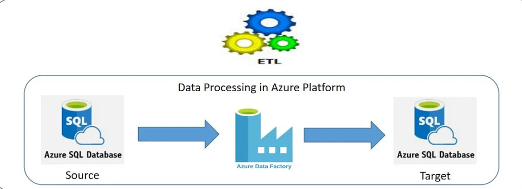
3. What is the difference between traditional ETL tools and Alteryx?
Traditional ETL or Extract, Transform, and Load tools can be limited in the types of data they can copy from one or more sources to the destination system. However with Alteryx’s unique metadata loader system, one could custom build a metadata loader to successfully copy over essentially any type of data, providing a unique advantage over other ETL tools. Alteryx of course comes with many metadata loaders already pre-built and ready to integrate into clients systems.
4. What are the Alteryx products in the Alteryx family and what do each do at a high level?
Alteryx Connect: a collaborative, data exploration and data cataloging platform for the enterprise that changes how information workers spend time finding new insights in the enterprise. Alteryx Connect empowers analysts and line-of-business users with the ability to easily and quickly find, understand, trust, and collaborate on the data that resides in their organization.
Alteryx Server: Alteryx Server provides a flexible and secure architecture that is designed to fit into your organization’s governance strategy. Built-in authentication, integrated SSO, and a granular permissions model provides enterprise-grade security.
Alteryx Designer: Empowers analysts and data scientists with a self-service data analytic experience to unlock answers from nearly any data source available with 250+ code-free and code-friendly tools. Using a repeatable drag-and-drop workflow, you can quickly profile, prepare and blend all of your data without having to write SQL code or custom scripts.
Alteryx Promote: Alteryx Promote makes developing, deploying, and managing predictive models and real-time decision APIs easier and faster. As an end-to-end data science model production system, Alteryx Promote allows data scientists and analytics teams to build, manage, and deploy predictive models to production faster—and more reliably—without writing any custom deployment code.
Alteryx Analytics Hub: Alteryx Analytics Hub makes it easy to provide analytic collaboration spaces for analysts, data scientists, and decision makers to work together and share actionable insights every day. Empowering analysts to automate mundane analytic tasks, reports, and big data analyses ensures that tough decisions can be made quickly. Alteryx Analytics Hub delivers self-service analytics across teams in a secure and governed analytics environment with central administration to ensure data is always is always accessible.
Alteryx Intelligence Suite: Alteryx Intelligence Suite helps you turn your data into smart decisions. Unlock meaningful insights in your semi-structured and unstructured text data and accurately estimate future business outcomes with code-free machine learning.
Alteryx Location & Business Insights: Alteryx Location and Business Insights are prepackaged datasets from trusted market providers for you to immediately transform any ordinary analysis to extraordinary. Combine and analyze your internal data with these valuable datasets via drag and drop tools to easily reveal key location, consumer and business insights without needing advanced expertise.
5. How about sharing a use case where we(you) were presented with a complex problem/obstacle and how we(you) found a creative way to overcome it using Alteryx?
My biggest accomplishment that utilized my business analysis and Alteryx skills was improving one quarterly model.
Pre state. 60 hours of work – the most significant delay in the production – 3 months. No proper documentation and no understanding of the process which involved using around 15 different data sources.
When my solution was ready, the model was on time, and it took me 20 hours to finalize model and prepare the documentation to handle the process to someone else.
How have I done it?
I worked with one of my colleagues to create a plan and understand what needs to be done to recreate the process. I spoke with various stakeholders to know if we still need all of the data sources. As the last step, I have rebuilt a process in Alteryx to make it easier to handle in the future.
6. What is Alteryx?
Alteryx is a powerful data analytics tool that allows users to blend, prepare, and analyze data from various sources quickly and easily. It’s designed to be user-friendly, enabling both technical and non-technical users to perform complex data operations without needing extensive coding knowledge. Here are some key features and functionalities of Alteryx:
Key Features:
1. Data Preparation and Blending:
- ETL (Extract, Transform, Load): Alteryx simplifies the process of extracting data from various sources, transforming it according to business requirements, and loading it into desired destinations.
- Data Cleaning: It offers tools to cleanse data, handle missing values, remove duplicates, and standardize data formats.
2. Analytics:
- Predictive Analytics: Alteryx includes built-in tools for predictive modelling, allowing users to forecast future trends and behaviours.
- Statistical Analysis: Users can perform various statistical analyses to understand data distributions, relationships, and insights.
3. Spatial Analytics:
- Geospatial Analysis: Alteryx can handle geolocation data, enabling users to perform spatial analyses such as mapping, distance calculations, and route optimizations.
4. Automation:
- Workflow Automation: Users can automate repetitive data processing tasks by creating workflows that can be scheduled to run at specific times or triggered by specific events.
- Integration: Alteryx integrates with various data sources and platforms, including databases, cloud services, APIs, and more.
5. Visualization and Reporting:
- Dashboards and Reports: Alteryx allows users to create interactive dashboards and reports to visualize data insights.
- Integration with BI Tools: It can integrate with business intelligence tools like Tableau and Power BI for advanced data visualization and reporting.
6. User-Friendly Interface:
- Drag-and-Drop Interface: Alteryx’s intuitive drag-and-drop interface makes it easy for users to build complex workflows without needing to write code.
- Pre-Built Tools: It offers a wide range of pre-built tools and connectors to handle various data processing tasks.
Use Cases:
- Data Preparation for Analysis: Cleaning and transforming raw data into a usable format for analysis.
- Marketing Analytics: Analyzing customer data to segment audiences, optimize campaigns, and predict customer behaviors.
- Supply Chain Optimization: Analysing supply chain data to optimize routes, reduce costs, and improve efficiency.
- Financial Analysis: Performing financial modelling, risk analysis, and forecasting.
Benefits:
- Efficiency: Speeds up data processing and analysis tasks, saving time and effort.
- Accessibility: Makes data analytics accessible to a broader range of users, including those without technical backgrounds.
- Integration: Seamlessly connects with various data sources and platforms, facilitating comprehensive data analysis.
Overall, Alteryx empowers organizations to turn data into actionable insights efficiently and effectively.
- Why do we use alteryx tool?
- Alteryx provide easily learnable solutions. Through these solutions organisation can quickly merge, analyze and prepare the data in the provided time irrespective of the business intelligence capabilities the employee perceives.
- Makes data analytics accessible to a broader range of users, including those without technical backgrounds.
- Seamlessly connects with various data sources and platforms, facilitating comprehensive data analysis.
What is alteryx server?
Alteryx Server is a platform that allows you to automate, share, and manage your data workflows and analytics across your organization. Here’s a simple explanation:
Alteryx Server: Key Points
1. Automation:
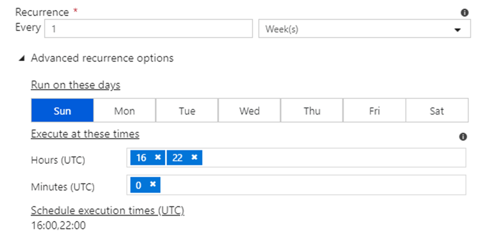
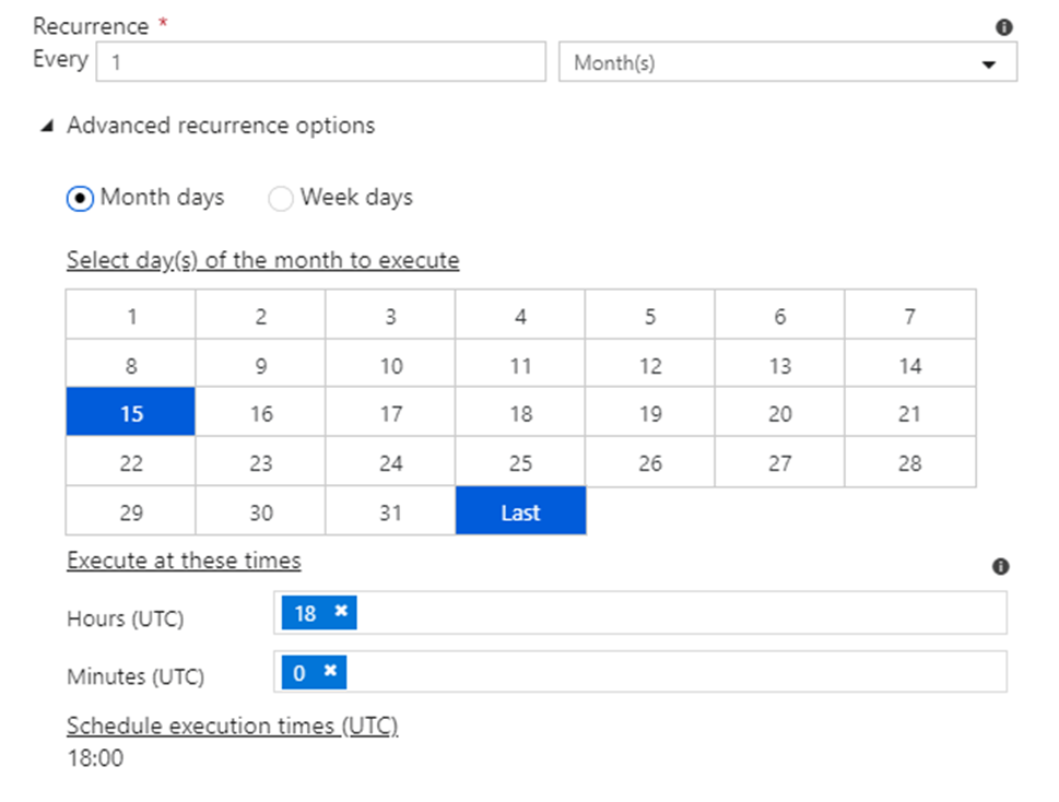
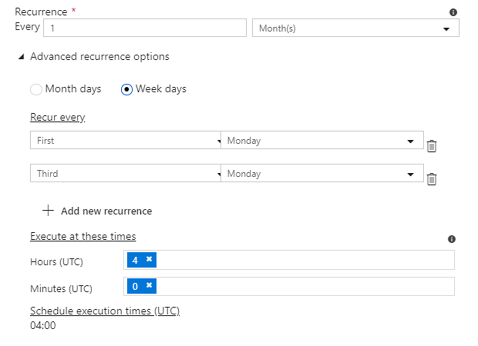
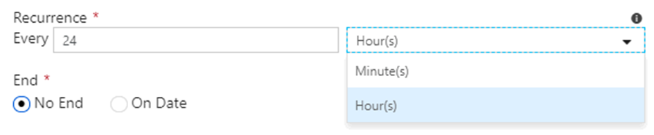
- Alteryx Server lets you schedule your data workflows to run automatically at specific times or intervals. This means you don’t have to manually run processes every time you need updated results.
2. Collaboration:
- Teams can share workflows and data analyses easily. With Alteryx Server, multiple users can access, run, and manage workflows from a central location, ensuring everyone is using the most current data and processes.
3. Scalability:
- It can handle large volumes of data and multiple users simultaneously. This makes it suitable for organizations with extensive data processing needs.
4. Centralized Management:
- All workflows, data connections, and results are stored in one place. This centralized system helps in maintaining consistency, security, and version control.
5. Web-Based Interface:
- Users can access and run workflows through a web interface. This makes it convenient to use Alteryx Server from any device with internet access, without needing to install any software locally.
Example Scenario:
Imagine you work for a company that needs to generate a daily sales report. Without Alteryx Server, you might have to manually run your workflow on your computer every day, save the results, and then email them to your team.
With Alteryx Server:
- Scheduling: You set up the workflow once and schedule it to run every morning at 6 AM.
- Automation: Alteryx Server automatically runs the workflow, processes the data, and generates the report.
- Access: Your team can log into the Alteryx Server web interface and access the latest report anytime they need it.
- Collaboration: If someone in your team updates the workflow, the changes are saved on the server, ensuring everyone works with the latest version.
In summary, Alteryx Server streamlines data processing, improves collaboration, and ensures your workflows are efficient and up-to-date, all through a centralized, automated system.

7. Explain some of the most important tools of Alteryx?
Alteryx is a powerful data preparation and analytics platform that offers a wide range of tools to help users process, analyze, and visualize data. Some of the most important tools in Alteryx include:
1. Input/Output Tools: These tools allow users to connect to various data sources (e.g., databases, files, APIs) to import and export data.

2. Preparation Tools: Alteryx provides a variety of tools for data cleansing, transformation, and enrichment. These include tools for filtering, sorting, joining, and aggregating data.

3. Spatial Tools: Alteryx has tools for working with spatial data, such as geocoding, spatial matching, and spatial analysis tools.

4. Predictive Tools: Alteryx offers a range of predictive analytics tools, including tools for building and validating predictive models.

5. Reporting and Visualization Tools: Alteryx allows users to create interactive reports and visualizations using tools like the Interactive Chart and Reporting tools.

6. Workflow Canvas: Alteryx’s workflow canvas is where users can drag and drop tools to build data workflows. It provides a visual representation of the data flow and allows users to easily connect and configure tools.

7. Data Investigation Tools: Alteryx provides tools for exploring and understanding data, such as the Browse tool, which allows users to inspect the data at various stages of the workflow.

8. Macro Tools: Macros in Alteryx allow users to create reusable workflows. They can be used to encapsulate complex logic or to create custom tools.

These are just a few examples of the tools available in Alteryx. The platform is highly customizable and extensible, allowing users to create a wide range of data processing and analysis workflows.
10. What are the different input file format supported in the alteryx?

11. What are the different database supported in the alteryx, which database have you connected in alteryx. How you will limit the number of rows retrieved?


These are some of important database you can connect, even your data source is not in the list you can always use generic connection ODBC to connect the same.
Limiting the Number of Rows Retrieved
- Using a SQL Query: When configuring the Input Data tool, you can write a custom SQL query to limit the number of rows.
- Using the Sample Tool: After retrieving the data, you can use the Sample tool in Alteryx to limit the number of rows. This tool allows you to specify the number of rows you want to keep or skip.
- Using the Input Data Tool Configuration: Some database connections in Alteryx allow you to set row limits directly within the Input Data tool configuration. Look for an option to limit rows when setting up your database connection.
12. Is there any limit on the number of rows and column retrieved from Alteryx?
Alteryx does not impose explicit limits on the number of rows or columns that can be retrieved or processed. However, there is a catch you can only read the data upto 2GB in a single set.
13. What are the best practices to handle Large Datasets?
To efficiently manage large datasets in Alteryx, consider the following best practices:
Filter and Sample Early: Apply filters and sampling early in your workflow to reduce the amount of data processed. This can help improve performance by focusing only on relevant data.
Use In-Database Tools: Alteryx provides In-Database tools that allow you to perform data processing within the database itself, leveraging the database’s processing power and reducing data movement.
Optimize Data Types: Use appropriate data types for your columns to minimize memory usage. For example, use integer types for numeric data when possible instead of floating-point types.
Batch Processing: If the dataset is too large to process in one go, consider splitting it into smaller batches and processing them sequentially or in parallel.
Monitor Resource Usage: Keep an eye on your system’s resource usage (CPU, memory, disk I/O) while running workflows to identify and address potential bottlenecks.
By following these practices, you can effectively manage large datasets in Alteryx and ensure that your workflows run efficiently.
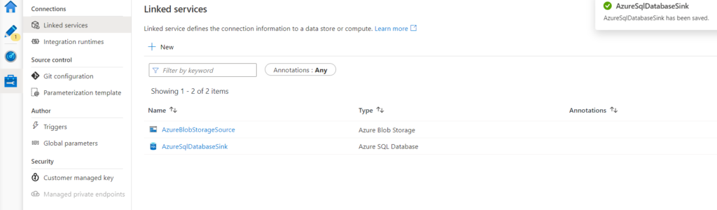
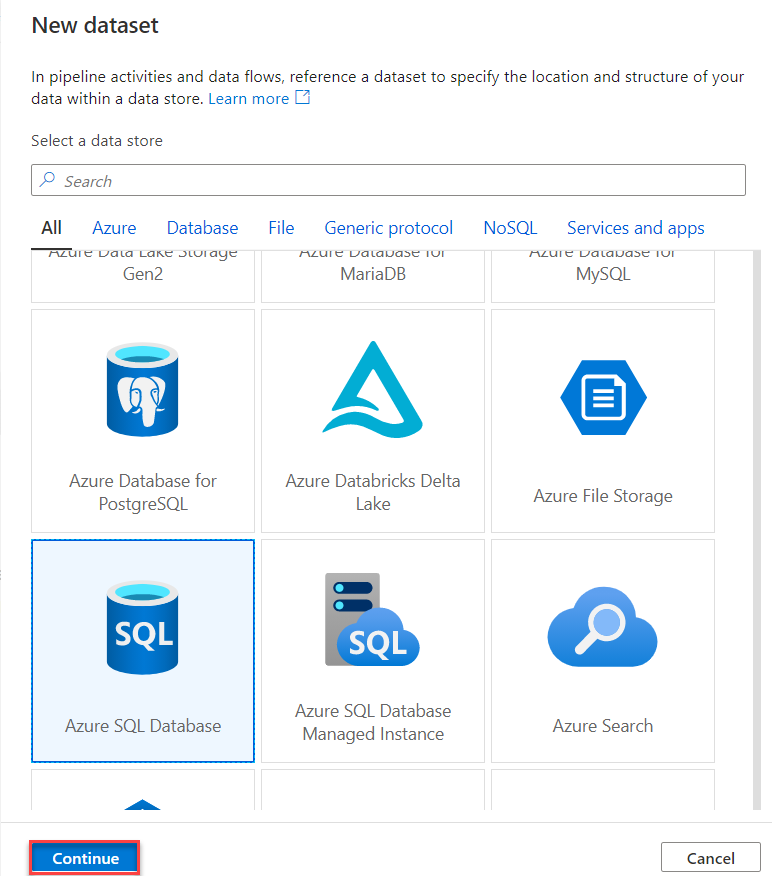
14. Can you write the table in the Database using alteryx, if yes which tool will you use. What will be the configuration of that tool?
Yes, you can write data to a database using Alteryx. The tool you would use for this purpose is the Output Data Tool.
Configuration of the Output Data Tool
Here is a step-by-step guide to configuring the Output Data Tool to write data to a database:
1. Drag and Drop the Output Data Tool:
- Drag the Output Data tool from the Tool Palette onto your workflow canvas.
2. Connect the Tool to Your Workflow:
- Connect the Output Data tool to the previous tool in your workflow that contains the data you want to write to the database.
3. Configure the Output Data Tool:
- In the Configuration window of the Output Data tool, specify the following settings:
Output Connection:
- Click on the drop-down menu next to the `Output Data` field and select `Database Connection`. Choose the appropriate database type (e.g., SQL Server, Oracle, MySQL, etc.).
Data Source Name (DSN) or Connection String:
- If you have a Data Source Name (DSN) configured for your database, select it from the list. Alternatively, you can specify a custom connection string to connect to your database.
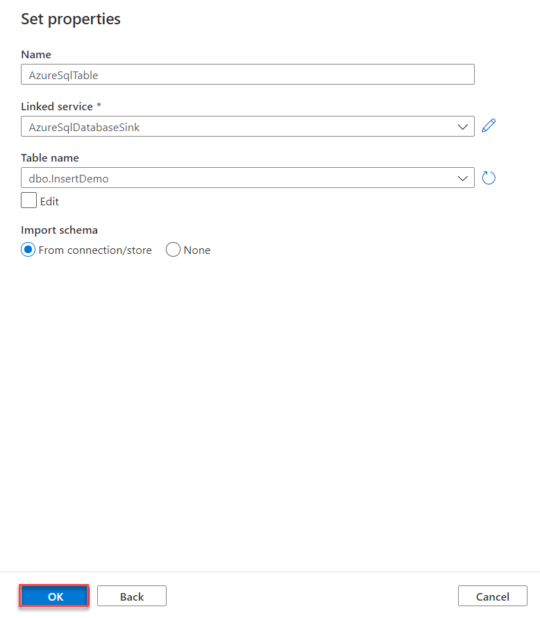
Table/Query:
- In the `Write to File or Database Table` field, specify the name of the table you want to write data to. You can type the table name directly or use the `Select Table` option to browse and select an existing table from your database.
- If the table does not exist, you can create a new table by typing the desired table name.
Options:
- Append Existing: Choose this option if you want to append data to an existing table.
- Overwrite Table (Drop): Choose this option if you want to drop the existing table and create a new one with the same name.
- Overwrite Table (Truncate): Choose this option if you want to truncate the existing table before inserting new data.
- Create Table: This option will create a new table if it does not already exist.
Field Map:
- Use this section to map the fields in your Alteryx data stream to the columns in the database table. Alteryx will automatically map fields based on matching names, but you can manually adjust the mappings if needed.
Additional Options:
- Depending on the database you are using, there may be additional configuration options available. For example, you can specify bulk insert options, specify primary keys, or set other database-specific settings.
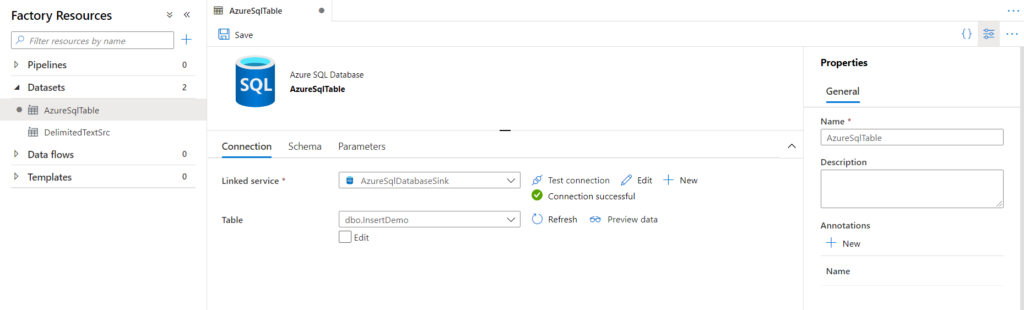
4. Test the Connection:
- Before running the workflow, it’s a good idea to test the database connection to ensure that Alteryx can connect to the database and write data.
5. Run the Workflow:
- Once everything is configured, run your workflow. Alteryx will write the data to the specified database table based on your configuration settings.
By following these steps, you can effectively write data to a database using Alteryx and the Output Data tool.
15. Which CRUD Operations in Database can you perform in Database?
Yes, we can do Crud operation in Database and following are the some of them:
- Create New Table
- Delete Data and append
- Overwrite Table (Drop)
- Update: insert if new
- Update: Warm on update failure
- Update: Error on update Failure.

16. Can you do the web scraping of data in alteryx?
Yes, following are the steps:

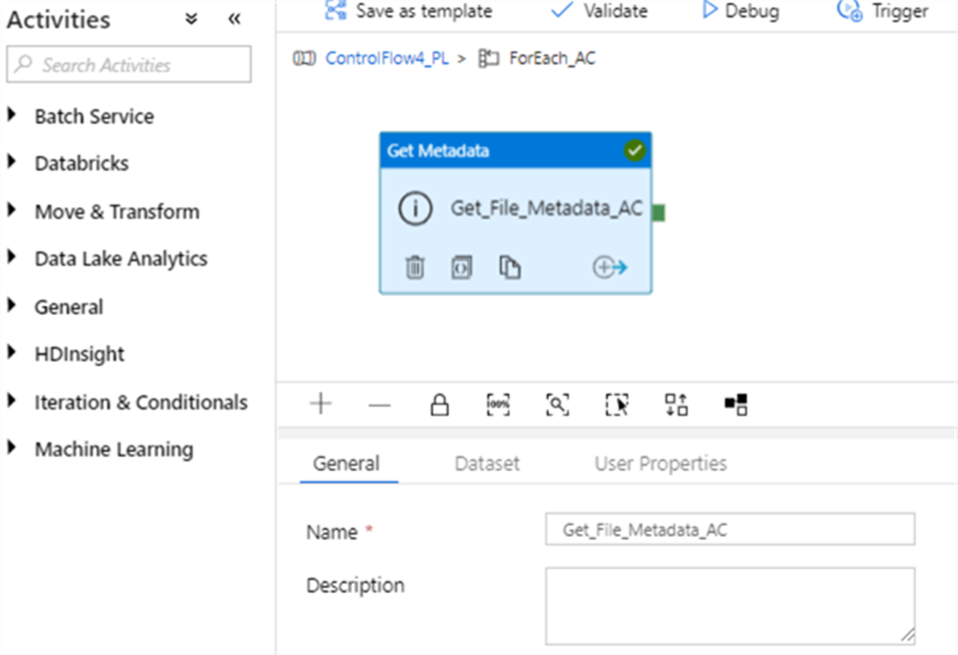
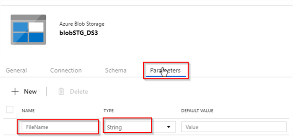
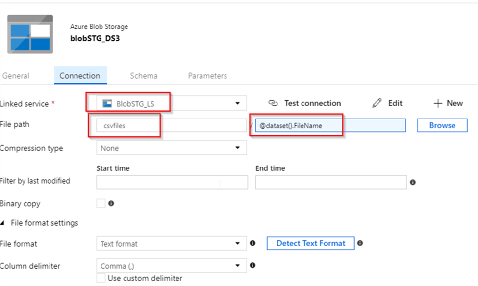
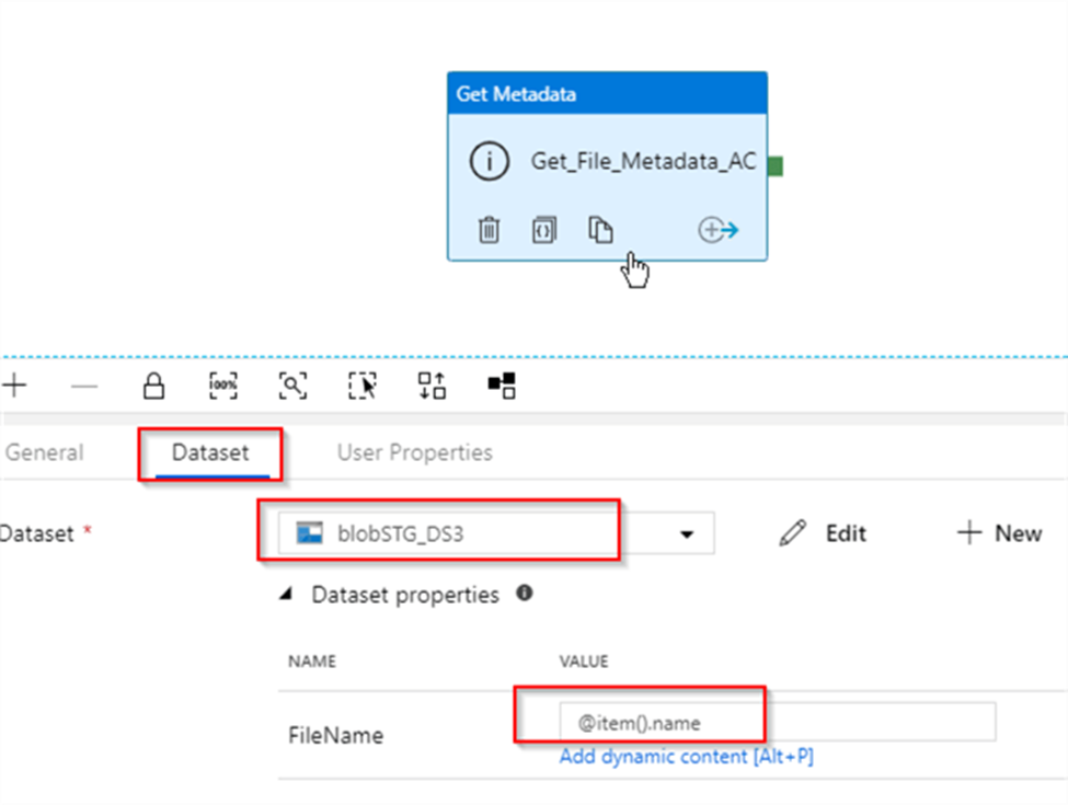
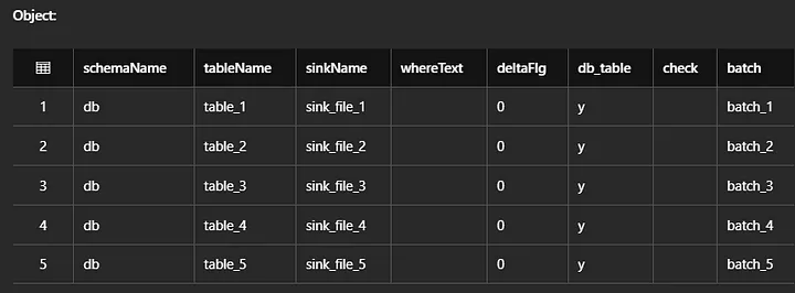
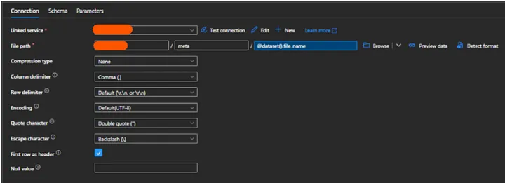
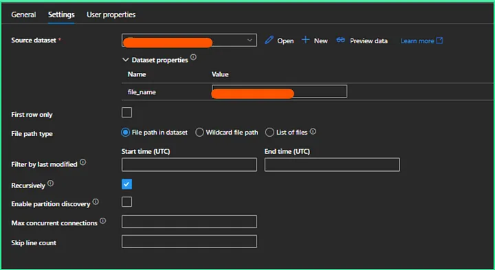
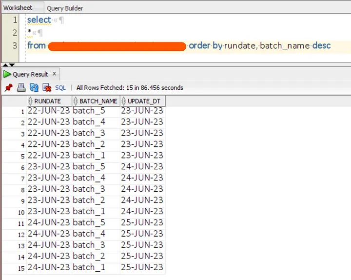
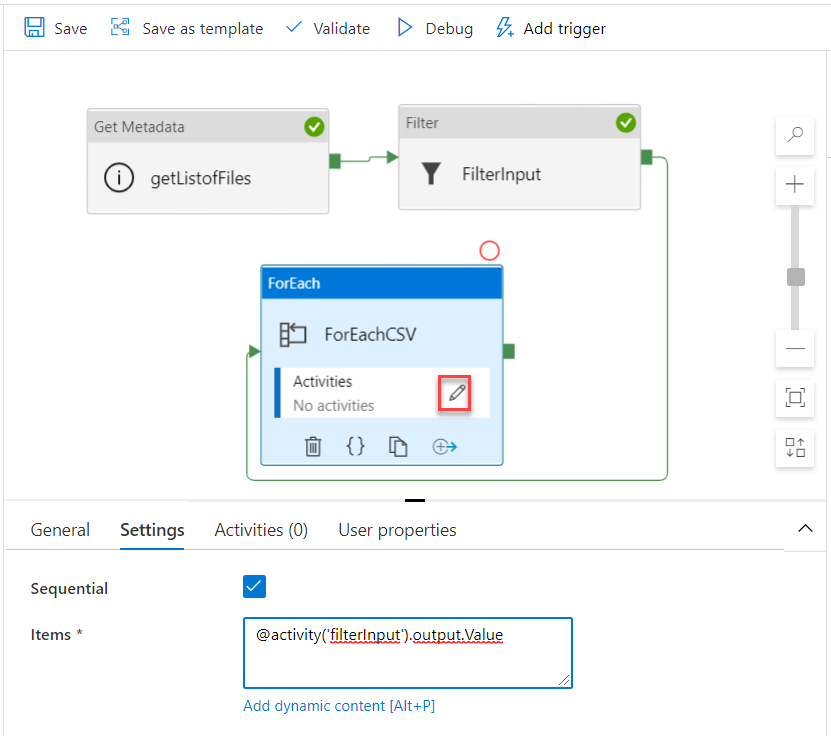
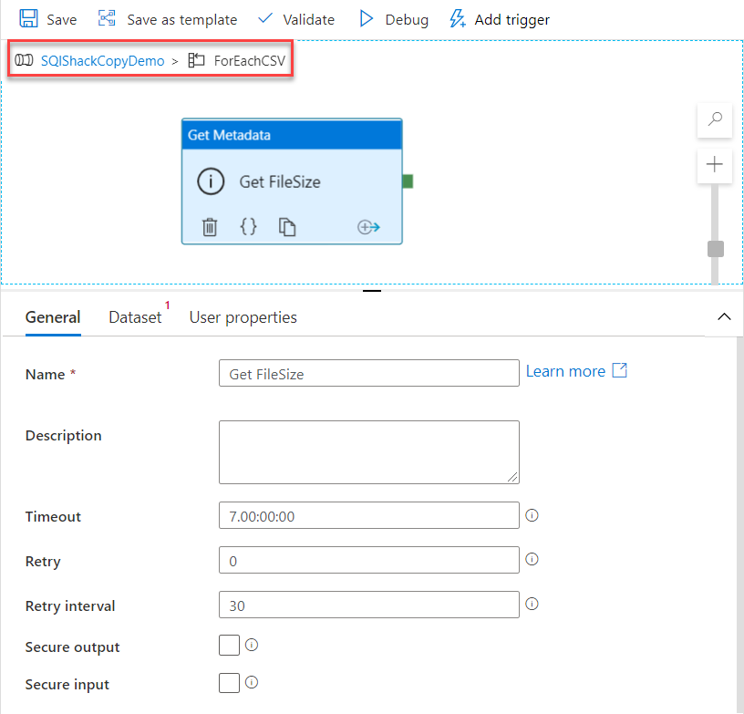
17. How you will read all the file present in the directory in?
To read all the files present in a directory in Alteryx, you can use a combination of the Directory Tool and the Dynamic Input Tool.
Directory Tool:
- Directory: C:\path\to\your\directory
- File Specification: *.csv
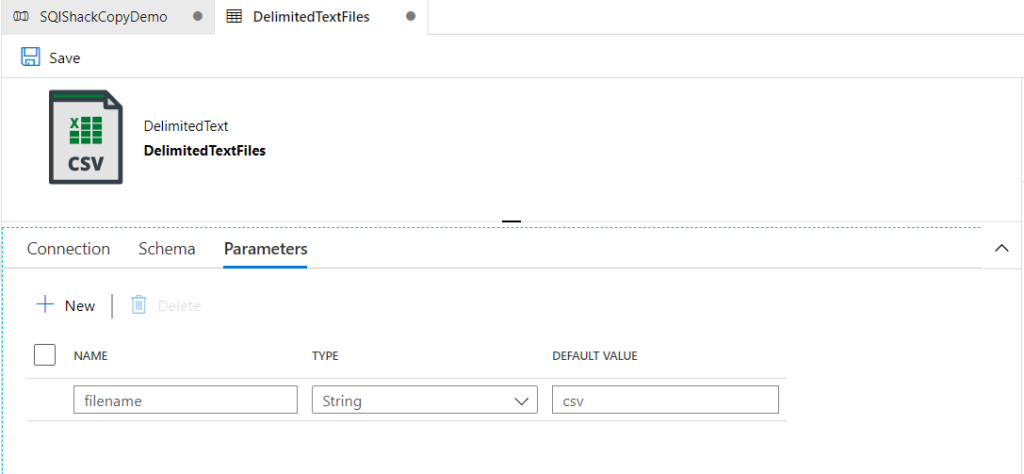
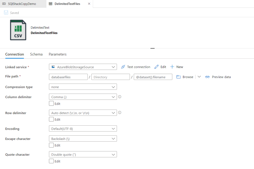
Dynamic Input Tool:
- Input Data Source Template: C:\path\to\your\directory\sample_file.csv
- File/Table Name: Full Path


18. What is configuration Pane in alteryx?
The Configuration Pane in Alteryx is the area where you configure the settings and properties of a selected tool in your workflow. It allows you to specify parameters, set options, and define how the tool should operate on the data. The configuration options vary depending on the specific tool you have selected, providing a tailored interface for customizing each tool’s functionality.
19. Is configuration Pane for a tool and interface same?
No, the Configuration Pane for a tool and the Interface are not the same in Alteryx.
Configuration Pane
– Purpose: The Configuration Pane is used to set up and customize the behavior and settings of individual tools in your workflow.
– Location: It is located on the left side of the Alteryx Designer interface.
– Functionality: When you select a tool in the workflow, the Configuration Pane displays the specific settings and options for that tool, allowing you to define how it processes data.
Interface
Purpose: The Interface refers to the entire user interface of Alteryx Designer, which includes various panes, tools, and options for building and managing workflows.
Components: The Interface includes several components, such as:
- Tool Palette: Where you can find and drag tools onto the canvas.
- Workflow Canvas: The central area where you build and visualize your workflows.
- Configuration Pane: Where you configure the selected tool.
- Results Pane: Where you view the output and logs of your workflow execution.
- Properties Window: Displays properties and metadata of the selected items.
In summary, the Configuration Pane is a specific part of the overall Alteryx interface focused on setting up individual tools, while the Interface encompasses the entire Alteryx Designer environment.
20. What you will do if your data start at row number 30 in excel?
In input tool configuration choose “Start data import on line” value as 30.

21. What is the difference between Unique tool and filter tool?
The Unique Tool and the Filter Tool in Alteryx serve different purposes and are used for different types of data processing tasks. Here are the key differences between them:
Summary of Differences:
| Feature | Unique Tool | Filter Tool |
| Purpose | Identify unique and duplicate records | Split data based on a condition |
| Outputs | Unique records, Duplicate records | True records, False records |
| Based On | Selected fields for uniqueness | User-defined condition or expression |
| Use Case | De-duplication, finding unique entries | Data segmentation, conditional filtering |
In summary, use the Unique Tool when you need to manage duplicate data and the Filter Tool when you need to segment your data based on specific conditions.
22. Can formula tool works on multiple stream of Data?
No, the Formula Tool in Alteryx does not work on multiple streams of data simultaneously. It is designed to operate on a single data stream at a time. The Formula Tool allows you to create new columns, update existing columns, or perform calculations and transformations on the data within a single input stream.
23. What is Multiple field binning tool?
The Multiple Field Binning Tool in Alteryx is used to categorize or bin continuous numerical data into discrete intervals, also known as bins or buckets, across multiple fields. This is particularly useful for segmenting data into ranges to facilitate analysis, reporting, or further data processing.

24. What is the difference between sample and random sample tool?
Summary of Differences
| Feature | Sample Tool | Random Sample Tool |
| Selection Method | Specific rows or percentages | Random rows or percentages |
| Selection Criteria | Based on position (first N, every Nth, etc.) | Random selection |
| Use Cases | Data validation, subset extraction | Random sampling for statistical analysis, testing models |
| Reproducibility | Not inherently random | Can be made reproducible with a seed value |
Example Scenarios:
Sample Tool: You have a dataset of 10,000 rows and want to analyze the first 100 rows to check data quality.
Random Sample Tool: You have a dataset of 10,000 rows and want to randomly select 1,000 rows to train a machine learning model.
By understanding these differences, you can choose the appropriate tool for your specific data sampling needs in Alteryx.
25. Is there any way to change Data type and size of the column?
Yes, using select operation we can do this operation.
26. Can you give me the practical scenario where you have used Multiple row formula?
Multiple Row Formula tool in Alteryx is used when you need to perform calculations that involve multiple rows of data at once, often to create rolling calculations or comparisons between rows. This tool allows you to reference values from previous or subsequent rows within the same calculation.
Here are some common use cases for the Multiple Row Formula tool:
1. Calculating running totals or cumulative sums: You can use the Multiple Row Formula tool to calculate running totals or cumulative sums for a specific column.
2. Calculating differences or changes between rows: For example, calculating the difference in sales between the current and previous days.
3. Calculating averages or other aggregate functions across multiple rows: You can use this tool to calculate moving averages or other aggregate functions that involve multiple rows.
4. Performing complex conditional calculations: If your calculation involves conditions that depend on values in multiple rows, the Multiple Row Formula tool can help you achieve this.
5. Calculating rates of change: You can use this tool to calculate rates of change between values in different rows, such as growth rates or percentage changes.
Overall, the Multiple Row Formula tool is useful for performing calculations that require referencing values from multiple rows within a dataset.
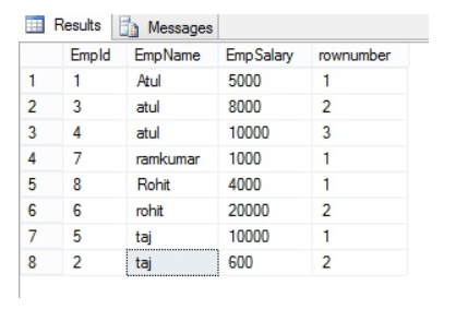
In below example we are creating Time Between calls by Employee

27. Can you update a existing sales with the last 3 months running Average of sales?
Yes, we can do that by using Multi Row formula
28. How you will refer back to 3-month sales data?
By using Num rows we can refer back.

29. I want to select the record number 100-1000 ? Tell me 3 different ways to do that?
- Combination of record Id and filter tool
- Using the limit options in input with import data at line. Basically you need to select Range at the time of input. But this option will only applicable for flat file.
- Using Select Records tool


30. Is Join tool part of Preparation Tool?
No, Join tool is not part of preparation tool.
31. Can grouping possible in Tile Tool?
Yes, its possible.

32. What Multiple tools are available in alteryx?
- Multi field binning tool
- Multi row formula
33. What are the available tool for multiple outstream in alteryx?
- Unique tool
- Filter tool
- Create sample tool
34. Which tool can change Data type or alter existing column in alteryx?
- Select Tool
- Multi row formula tool
35. What is difference between the join and join multiple tool?
In Alteryx, both the Join and Join Multiple tools are used to combine data from different sources, but they have different functionalities and use cases:
Join Tool:
The Join tool is used to combine two data streams based on a common field or fields. Here are some key features and functionalities:
- Input Anchors: It has two input anchors: Left (`L`) and Right (`R`).
- Join Conditions: You can specify one or more fields to join on from each input.
- Output Anchors: It has three output anchors:
- `J`: Rows that match on the join fields from both inputs.
- `L`: Rows that are unique to the left input.
- `R`: Rows that are unique to the right input.
Use Case:
Ideal for combining data from two sources where there is a clear relationship between them, such as combining customer information from two different systems using a common customer ID.
Join Multiple Tool
The Join Multiple tool is used to combine three or more data streams based on a common field or fields. Here are some key features and functionalities:
- Input Anchors: It has multiple input anchors (`Input 1`, `Input 2`, `Input 3`, etc.).
- Join Conditions: You can specify one or more fields to join on from each input.
- Output Anchor: It has a single output anchor that contains the combined data.
Use Case:
Ideal for combining multiple data sources where each source shares a common field or fields, such as merging data from different departments that all use a common identifier like employee ID or product code.
Summary
- Join Tool: Best for joining two data streams with options to output matching and non-matching records separately.
- Join Multiple Tool: Best for joining three or more data streams into a single output based on common fields.
Both tools are essential in data blending and preparation workflows in Alteryx, offering flexibility depending on the complexity and requirements of the data joining task.
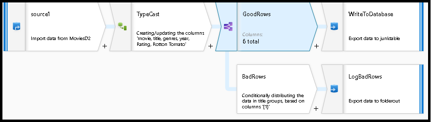
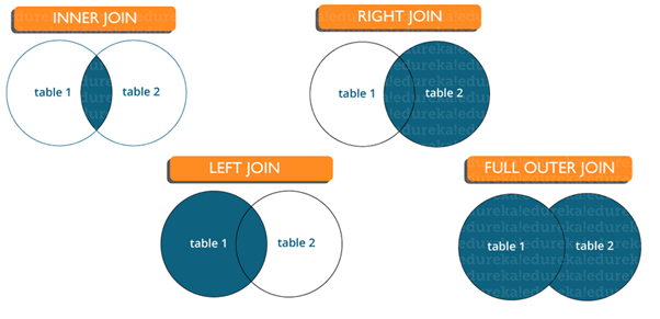
36. How can you create the full join in alteryx?
Here’s a visual representation of the workflow steps:
Join Tool Configuration:
- Input 1: Left Dataset
- Input 2: Right Dataset
- Join on: Common Field
Union Tool Configuration:
- Input 1: J (Join output)
- Input 2: L (Left output)
- Input 3: R (Right output)
Result:
The Union tool will produce a combined dataset that includes all records from both input datasets, representing a full join.
By following these steps, you effectively create a full join in Alteryx, ensuring that all records from both input datasets are included in the final output, whether they have matching join keys or not.
37. What are the usages of make group tool/ Fuzzy match tool?
- Make Group Tool: Used for clustering similar records within a dataset based on specified fields and similarity thresholds. It helps in grouping and categorizing records for further analysis.
- Fuzzy Match Tool: Used for matching records from different datasets or within the same dataset based on approximate matches. It is valuable for data cleansing, deduplication, and linking related records.
Both tools enhance the ability to work with imperfect or inconsistent data by providing mechanisms to identify and group similar or related records effectively.
38. How many tables can you join and can you perform and can you perform a join between a excel and a Databases?
In Alteryx, you can join multiple tables, and it is possible to perform joins between different data sources, including Excel files and databases.
39. Which file will be given preference in union operation?
Its totally depend on the configuration at the time of union operation. Find following screen shot for your reference.

40. Which tool can perform VLOOKUP operation in alteryx?
Find and Replace tool is used for Vlookup operation in alteryx.

41. What all operation a Find and Replace tool can perform?
Following operation it can perform:
- Replace the starting of the string with specified text.
- Replace whole string with column in source dataset.
- Replace character from anywhere in the string.

42. What is the difference between the Crosstab and Transpose tool?
Crosstab Tool:
Converts rows to columns, used for pivoting data from a long to a wide format. Ideal for creating summary tables and pivot tables.
Example:
- Input: Sales data with columns for Region, Product, and SalesAmount.
- Output: A table where each row represents a region, each column represents a product, and the cells contain the total sales amount for each product in each region.
Transpose Tool:
Converts columns to rows, used for unpivoting data from a wide to a long format. Ideal for normalizing and reshaping data for further analysis.
Understanding the difference between these tools helps in selecting the appropriate one for your data transformation needs in Alteryx.
Example:
- Input: Sales data with columns for Region, ProductA_Sales, ProductB_Sales.
- Output: A table with columns Region, Product, and SalesAmount, where each row represents the sales amount for a specific product in a specific region.

43. What is the wide Data and what is Tall Data?
Wide Data:
Each entity is a single row, with different measurements in separate columns. Suitable for comparison across variables for the same entity.
| Region | ProductA_Sales | ProductB_Sales | ProductC_Sales |
| North | 100 | 150 | 200 |
| South | 80 | 120 | 160 |
| East | 90 | 110 | 140 |
| West | 70 | 130 | 170 |
Tall (Long) Data:
Each measurement is a separate row, with fewer columns. Suitable for detailed analysis, time series data, and certain statistical methods.
| Region | Product | SalesAmount |
| North | ProductA | 100 |
| North | ProductB | 150 |
| North | ProductC | 200 |
| South | ProductA | 80 |
| South | ProductB | 120 |
| South | ProductC | 160 |
| East | ProductA | 90 |
| East | ProductB | 110 |
Choosing between wide and tall formats depends on the analysis or visualization you plan to perform. Tools like the Crosstab and Transpose tools in Alteryx help convert data between these formats to suit different needs.
44. How can you use crosstab or Transpose tool to restructure the data and then move it to original format?
To restructure data using the Crosstab and Transpose tools in Alteryx and then revert it back to its original format, you need to understand how these tools transform data.
Example Scenario:
Suppose you have sales data in a long format that you want to convert to a wide format using the Crosstab tool.
Original (Tall) Data Format:
| Region | Product | SalesAmount |
| North | ProductA | 100 |
| North | ProductB | 150 |
| North | ProductC | 200 |
| South | ProductA | 80 |
| South | ProductB | 120 |
| South | ProductC | 160 |
- Using Crosstab Tool
- Group Data By: Region
- New Column Headers: Product
- Values for New Columns: SalesAmount
- Converts data from tall to wide format.
Output (Wide) Data Format:
| Region | ProductA | ProductB | ProductC |
| North | 100 | 150 | 200 |
| South | 80 | 120 | 160 |
- Using Transpose Tool:
- Key Columns: Region
- Data Columns to Transpose: ProductA, ProductB, ProductC
- Converts data back from wide to tall format.
Reverted (Tall) Data Format:
| Region | Name | Value |
| North | ProductA | 100 |
| North | ProductB | 150 |
| North | ProductC | 200 |
| South | ProductA | 80 |
| South | ProductB | 120 |
| South | ProductC | 160 |
By using these steps, you can effectively restructure your data into different formats and then revert it back to its original structure using the Crosstab and Transpose tools in Alteryx.
45. What is the use of count record tool?
The Count Records tool in Alteryx is essential for validating, monitoring, and controlling data workflows by providing a quick and reliable count of records in a dataset. Its simplicity and utility make it a valuable tool in ensuring the integrity and efficiency of data processing in Alteryx workflows.
Example Scenario
Input Data:
| ID | Name | Value |
| 1 | A | 10 |
| 2 | B | 20 |
| 3 | C | 30 |
Workflow with Count Records Tool:
Step 1: Connect the input data to the Count Records tool.
Step 2: Run the workflow.
Step 3: The Count Records tool outputs a single value indicating the number of records (in this case, 3).
46. What are the operation you can perform in summaries tool?
There are many operations you can do, some of them are like Group by, Count average etc.

47. Which tool can perform the Transform operation with Grouping?
Following are some of tool to achieve the same
- Arrange tool
- Cross Tab tool
- Summarize too
- Running Total
48. What are the macros and how they are different from normal workflow?
In Alteryx, macros are specialized workflows designed to be reusable components within other workflows. They help streamline repetitive tasks, encapsulate complex processes, and maintain consistency across multiple workflows. Here’s a detailed explanation of macros and how they differ from normal workflows:
Macros:
Definition:
Macros in Alteryx are reusable workflows that can be inserted into other workflows as a single tool. They are designed to perform specific tasks and can be parameterized to handle different inputs and configurations.
Types of Macros:
- Standard Macros: Basic reusable workflows that can be used to perform common tasks.
- Batch Macros: Run multiple iterations over an incoming dataset, processing each batch of data separately.
- Iterative Macros: Repeatedly process data until a specified condition is met, useful for recursive tasks.
- Location Optimizer Macros: Specialized macros for location-based optimization tasks.
Uses:
- Reusability: Encapsulate frequently used processes to avoid duplicating logic across multiple workflows.
- Maintainability: Simplify complex workflows by breaking them down into smaller, manageable components.
- Parameterization: Create flexible workflows that can handle varying inputs and configurations through the use of macro inputs and outputs.
| Feature | Normal Workflows | Macros |
| Purpose | Perform specific, single-use tasks or analyses | Encapsulate reusable processes or tasks |
| Reusability | Typically used once or occasionally | Designed to be reused across multiple workflows |
| Encapsulation | Entire sequence of operations included | Specific operations encapsulated within the macro, used as a single tool in workflows |
| Parameterization | Generally fixed, requires manual changes for different scenarios | Can accept inputs and parameters, making them flexible and adaptable |
| Workflow Complexity | Can become complex and hard to manage as they grow | Helps reduce complexity by modularizing workflows |
| Deployment | Deployed as standalone workflows | Deployed as tools within other workflows |
| Creation | Built and saved as a workflow (.yxmd) | Built and saved with specific macro extensions (.yxmc for standard, batch, iterative) |
| Configuration | Fixed configuration | Configurable inputs and outputs, allowing for different use cases |
| Examples | Data cleaning, reporting, analysis | Common data transformations, reusable calculations, parameterized operations |
| Tool Integration | Standard tools and operations | Custom tools created by combining standard tools and operations |
Example Scenario
Normal Workflow:
- A workflow that reads data, filters it, performs calculations, and generates a report.
Macro Workflow:
- A macro that performs a specific calculation or data transformation, which can be reused in multiple reporting workflows.

49. What is the Interface designer and what does it do?
The Interface Designer in Alteryx is a powerful tool that allows you to create custom user interfaces (UIs) for your workflows. It enables you to build interactive applications that can be used by non-technical users to input data, configure settings, and visualize results.
Benefits of Using the Interface Designer:
- User-Friendly: Allows non-technical users to interact with workflows without needing to understand the underlying logic.
- Customization: Create tailored interfaces for specific tasks or users.
- Efficiency: Streamline data input and processing by guiding users through the workflow.
- Interactivity: Enable users to explore data and make informed decisions through interactive controls and visualizations.
- Automate repetitive tasks and workflows by providing a structured interface for input and output.
Example Use Cases:
Data Preparation:
Allow users to select datasets, set filters, and specify data cleaning operations.
Data Analysis:
Provide options for selecting variables, choosing analysis methods, and viewing results in charts or tables.
Reporting:
Create interfaces for generating customized reports with user-specified parameters.
Workflow Orchestration:
Build interfaces for managing and monitoring complex workflows, with options to start, pause, or stop processes.
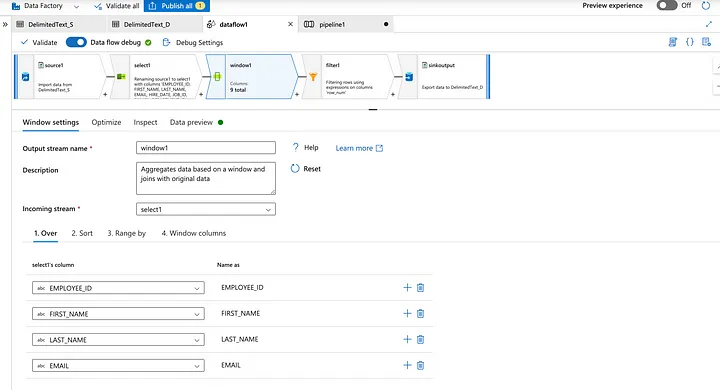
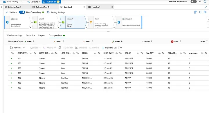
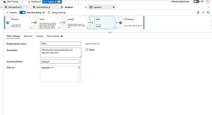
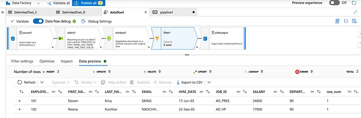
This workflow demonstrates data analysis, transformation and reporting similar to typical operations of financial analysts. Calculate typical KPIs such as Year over Year and YTD calculations for departments.

50. Can you take the field name as input of the interface tool?
Yes, drop down and list box can take the field name as input, not other tool.


51. What is control parameter and what is action, how you can differentiate between them?
- Control Parameter: Collects user input or configures settings.
- Action: Triggers a specific behaviour or operation within the workflow.
Differentiation
- Purpose: Control parameters are used to collect user input or configure settings, while actions are used to trigger specific behaviors or operations within the workflow.
- Interaction: Control parameters interact with users to gather information, while actions interact with the workflow to perform tasks.
- Representation: Control parameters are typically input elements (e.g., text boxes, dropdowns), while actions are often buttons or interactive elements that trigger a response.
52. What are the various Interface tool?
In Alteryx, the Interface tools are used in the Interface Designer to create custom user interfaces for workflows. These tools allow you to design interactive forms and controls that users can interact with to provide input, configure settings, and view results. Here are the main Interface tools available in Alteryx:
- Action Tool: Executes an action when triggered, such as running a workflow or updating data.
- Control Parameter Tool
- Checkbox Tool: Allows users to select or deselect an option, which can trigger actions or change settings.
- Date Picker Tool: Provides a calendar interface for users to select a date, which can be used as input for date-based operations.
- Dropdown Tool: Creates a dropdown list of options for users to select from.
- List Box Tool: Allows users to select one or more items from a list of options.
- Radio Button Tool: Presents a set of mutually exclusive options as radio buttons for users to select from.
- Textbox Tool: Displays text within the interface for instructional or informational purposes
- Toggle Tool: Creates a toggle switch for users to turn an option on or off.
These Interface tools provide a wide range of options for creating interactive and user-friendly interfaces for Alteryx workflows, enabling users to interact with data and workflows in meaningful ways.


53. What are the different action type available in the Action tool?
The options depend on the selected interface tool, it can vary as per the selected tool.
54. What are the different Geo location data types used in alteryx?
In Alteryx, the geolocation data types are used to represent geographic locations, such as latitude and longitude coordinates, as well as other location-related information. These data types are commonly used in spatial analysis and mapping applications. Here are the main geolocation data types in Alteryx:
1. Spatial Object (SpatialObj): This data type represents a spatial object, such as a point, line, or polygon, in a geographic coordinate system. Spatial objects can be used to represent geographic features, such as cities, roads, or boundaries.
2. Spatial Object (MultiObj): This data type represents a collection of spatial objects, such as a multi-point, multi-line, or multi-polygon, in a geographic coordinate system. MultiObj objects can be used to represent complex geographic features that consist of multiple parts.
3. Latitude (double): This data type represents the latitude coordinate of a point on the Earth’s surface. The latitude values range from -90 degrees (South Pole) to +90 degrees (North Pole).
4. Longitude (double): This data type represents the longitude coordinate of a point on the Earth’s surface. The longitude values range from -180 degrees (West of the Prime Meridian) to +180 degrees (East of the Prime Meridian).
5. Geohash (string): This data type represents a geohash, which is a compact representation of a geographic location. Geohashes are used to encode latitude and longitude coordinates into a short string, which can be useful for indexing and querying spatial data.
6. Spatial Reference (spatialref): This data type represents a spatial reference system (SRS), which defines the coordinate system used to represent geographic locations. Spatial reference systems can be used to convert between different coordinate systems and perform spatial calculations.
These geolocation data types in Alteryx provide the foundation for working with geographic data and performing spatial analysis and mapping tasks.
55. What are the different alteryx offered products?
Alteryx offers a range of products designed to assist with data analytics, data preparation, and data science workflows. Here are the key Alteryx products:
1. Alteryx Designer
- Description: The core product for data preparation, blending, and analytics.
- Features:
- Drag-and-drop interface for building workflows.
- Tools for data blending, cleansing, and transformation.
- Built-in predictive analytics and spatial tools.
- Integration with various data sources (databases, files, cloud services).
2. Alteryx Server
- Description: A platform for sharing and running analytic workflows at scale.
- Features:
- Centralized collaboration and sharing of workflows.
- Automated scheduling and execution of workflows.
- Web-based gallery for publishing workflows.
- API support for integrating with other systems.
3. Alteryx Connect
- Description: A data catalog and collaboration platform.
- Features:
- Discovery and sharing of data assets across the organization.
- Metadata management and data lineage tracking.
- Collaboration features like tagging, rating, and commenting on data assets.
4. Alteryx Promote
- Description: A platform for deploying and managing predictive models.
- Features:
- Model deployment and versioning.
- REST API for model scoring and integration.
- Monitoring and management of model performance.
- Support for models built in various tools (Alteryx Designer, R, Python).
5. Alteryx Intelligence Suite
- Description: An add-on to Alteryx Designer that enhances machine learning and text mining capabilities.
- Features:
- Automated machine learning tools.
- Natural language processing (NLP) tools.
- Computer vision tools for image processing.
- Enhanced data insights and visualizations.
6. Alteryx Data Packages
- Description: Curated data sets for specific industries and use cases.
- Features:
- Pre-packaged data sets ready for use in analytics workflows.
- Industry-specific data packages (e.g., demographics, consumer data).
- Regular updates and maintenance of data sets.
7. Alteryx Analytics Hub
- Description: A collaborative analytics environment for sharing and managing analytic workflows.
- Features:
- Centralized repository for workflows and data assets.
- Role-based access control and security.
- Integration with cloud storage and data sources.
- Collaboration features like workflow sharing and commenting.
These products cater to different aspects of the data analytics lifecycle, from data preparation and blending to advanced analytics and collaboration. Together, they provide a comprehensive suite of tools for organizations looking to enhance their data-driven decision-making processes.