Tag interview questions and answer

1. Why would an organization use a tool like Alteryx? Which capabilities, business problems could it solve for? 

The value prop and capabilities for any organization using Alteryx would be the fact that it supports better and faster decisions (social, collaborative and easy-to-use portal improves insights, analysis, and decision making). It Improves collaboration (retain tribal knowledge that exists within the organization and connect with others to help enrich the information being shared). Improves analytic productivity (reduce time spent searching for impactful and relevant data assets, and get to insights faster). No more waiting for emails with attached excel sheets of data that you have no idea where it’s been or the last time it has been updated.

2. Can you explain a scenario where a customer / end user would need Alteryx / Tableau? How could these tools be used together to provide value?

A analyst has been tasked with finding a report that has been outdated but is required to be used to compare to a current report and displayed graphically in Tableau. Rather than exchange numerous emails stretching over potentially many days with team members, IT, and management personnel, the analyst can go through Alteryx Connect search for the old report, tag it, and share it with the the analyst in charge of creating a graphical comparison of the report in Tableau. Once that graphic is completed it is automatically loaded into Alteryx Connect so that their entire team and whomever has access to it can view it. This significantly reduces turn around time for producing, sharing, and collaborating on reports. 

3. What is the difference between traditional ETL tools and Alteryx?

Traditional ETL or Extract, Transform, and Load tools can be limited in the types of data they can copy from one or more sources to the destination system. However with Alteryx’s unique metadata loader system, one could custom build a metadata loader to successfully copy over essentially any type of data, providing a unique advantage over other ETL tools. Alteryx of course comes with many metadata loaders already pre-built and ready to integrate into clients systems. 

4. What are the Alteryx products in the Alteryx family and what do each do at a high level? 

Alteryx Connect: a collaborative, data exploration and data cataloging platform for the enterprise that changes how information workers spend time finding new insights in the enterprise. Alteryx Connect empowers analysts and line-of-business users with the ability to easily and quickly find, understand, trust, and collaborate on the data that resides in their organization. 

Alteryx Server: Alteryx Server provides a flexible and secure architecture that is designed to fit into your organization’s governance strategy. Built-in authentication, integrated SSO, and a granular permissions model provides enterprise-grade security.

Alteryx Designer: Empowers analysts and data scientists with a self-service data analytic experience to unlock answers from nearly any data source available with 250+ code-free and code-friendly tools. Using a repeatable drag-and-drop workflow, you can quickly profile, prepare and blend all of your data without having to write SQL code or custom scripts.

Alteryx Promote: Alteryx Promote makes developing, deploying, and managing predictive models and real-time decision APIs easier and faster. As an end-to-end data science model production system, Alteryx Promote allows data scientists and analytics teams to build, manage, and deploy predictive models to production faster—and more reliably—without writing any custom deployment code.

Alteryx Analytics Hub: Alteryx Analytics Hub makes it easy to provide analytic collaboration spaces for analysts, data scientists, and decision makers to work together and share actionable insights every day. Empowering analysts to automate mundane analytic tasks, reports, and big data analyses ensures that tough decisions can be made quickly. Alteryx Analytics Hub delivers self-service analytics across teams in a secure and governed analytics environment with central administration to ensure data is always is always accessible.

Alteryx Intelligence Suite: Alteryx Intelligence Suite helps you turn your data into smart decisions. Unlock meaningful insights in your semi-structured and unstructured text data and accurately estimate future business outcomes with code-free machine learning.

Alteryx Location & Business Insights: Alteryx Location and Business Insights are prepackaged datasets from trusted market providers for you to immediately transform any ordinary analysis to extraordinary. Combine and analyze your internal data with these valuable datasets via drag and drop tools to easily reveal key location, consumer and business insights without needing advanced expertise.

5. How about sharing a use case where we(you) were presented with a complex problem/obstacle and how we(you) found a creative way to overcome it using Alteryx?

My biggest accomplishment that utilized my business analysis and Alteryx skills was improving one quarterly model.

Pre state. 60 hours of work – the most significant delay in the production – 3 months. No proper documentation and no understanding of the process which involved using around 15 different data sources.

When my solution was ready, the model was on time, and it took me 20 hours to finalize model and prepare the documentation to handle the process to someone else.

How have I done it?

I worked with one of my colleagues to create a plan and understand what needs to be done to recreate the process. I spoke with various stakeholders to know if we still need all of the data sources. As the last step, I have rebuilt a process in Alteryx to make it easier to handle in the future.

6. What is Alteryx?

Alteryx is a powerful data analytics tool that allows users to blend, prepare, and analyze data from various sources quickly and easily. It’s designed to be user-friendly, enabling both technical and non-technical users to perform complex data operations without needing extensive coding knowledge. Here are some key features and functionalities of Alteryx:

Key Features:

1. Data Preparation and Blending:

•  ETL (Extract, Transform, Load): Alteryx simplifies the process of extracting data from various sources, transforming it according to business requirements, and loading it into desired destinations.

• Data Cleaning: It offers tools to cleanse data, handle missing values, remove duplicates, and standardize data formats.

2. Analytics:

• Predictive Analytics: Alteryx includes built-in tools for predictive modelling, allowing users to forecast future trends and behaviours.

• Statistical Analysis: Users can perform various statistical analyses to understand data distributions, relationships, and insights.

3. Spatial Analytics:

• Geospatial Analysis: Alteryx can handle geolocation data, enabling users to perform spatial analyses such as mapping, distance calculations, and route optimizations.

4. Automation:

• Workflow Automation: Users can automate repetitive data processing tasks by creating workflows that can be scheduled to run at specific times or triggered by specific events.

• Integration: Alteryx integrates with various data sources and platforms, including databases, cloud services, APIs, and more.

5. Visualization and Reporting:

• Dashboards and Reports: Alteryx allows users to create interactive dashboards and reports to visualize data insights.

• Integration with BI Tools: It can integrate with business intelligence tools like Tableau and Power BI for advanced data visualization and reporting.

6. User-Friendly Interface:

• Drag-and-Drop Interface: Alteryx’s intuitive drag-and-drop interface makes it easy for users to build complex workflows without needing to write code.
• Pre-Built Tools: It offers a wide range of pre-built tools and connectors to handle various data processing tasks.

Use Cases:

• Data Preparation for Analysis: Cleaning and transforming raw data into a usable format for analysis.

• Marketing Analytics: Analyzing customer data to segment audiences, optimize campaigns, and predict customer behaviors.

• Supply Chain Optimization: Analysing supply chain data to optimize routes, reduce costs, and improve efficiency.

• Financial Analysis: Performing financial modelling, risk analysis, and forecasting.

Benefits:

• Efficiency: Speeds up data processing and analysis tasks, saving time and effort.

• Accessibility: Makes data analytics accessible to a broader range of users, including those without technical backgrounds.
• Integration: Seamlessly connects with various data sources and platforms, facilitating comprehensive data analysis.

Overall, Alteryx empowers organizations to turn data into actionable insights efficiently and effectively.

• Why do we use alteryx tool?
• Alteryx provide easily learnable solutions. Through these solutions organisation can quickly merge, analyze and prepare the data in the provided time irrespective of the business intelligence capabilities the employee perceives.
• Makes data analytics accessible to a broader range of users, including those without technical backgrounds.
• Seamlessly connects with various data sources and platforms, facilitating comprehensive data analysis.

What is alteryx server?

Alteryx Server is a platform that allows you to automate, share, and manage your data workflows and analytics across your organization. Here’s a simple explanation:

Alteryx Server: Key Points

1. Automation:

•  Alteryx Server lets you schedule your data workflows to run automatically at specific times or intervals. This means you don’t have to manually run processes every time you need updated results.

2. Collaboration:

• Teams can share workflows and data analyses easily. With Alteryx Server, multiple users can access, run, and manage workflows from a central location, ensuring everyone is using the most current data and processes.

3. Scalability:

• It can handle large volumes of data and multiple users simultaneously. This makes it suitable for organizations with extensive data processing needs.

4. Centralized Management:

• All workflows, data connections, and results are stored in one place. This centralized system helps in maintaining consistency, security, and version control.

5. Web-Based Interface:

• Users can access and run workflows through a web interface. This makes it convenient to use Alteryx Server from any device with internet access, without needing to install any software locally.

Example Scenario:

Imagine you work for a company that needs to generate a daily sales report. Without Alteryx Server, you might have to manually run your workflow on your computer every day, save the results, and then email them to your team.

With Alteryx Server:

• Scheduling: You set up the workflow once and schedule it to run every morning at 6 AM.

• Automation: Alteryx Server automatically runs the workflow, processes the data, and generates the report.

• Access: Your team can log into the Alteryx Server web interface and access the latest report anytime they need it.

• Collaboration: If someone in your team updates the workflow, the changes are saved on the server, ensuring everyone works with the latest version.

In summary, Alteryx Server streamlines data processing, improves collaboration, and ensures your workflows are efficient and up-to-date, all through a centralized, automated system.

7. Explain some of the most important tools of Alteryx?

Alteryx is a powerful data preparation and analytics platform that offers a wide range of tools to help users process, analyze, and visualize data. Some of the most important tools in Alteryx include:

1. Input/Output Tools: These tools allow users to connect to various data sources (e.g., databases, files, APIs) to import and export data.

2. Preparation Tools: Alteryx provides a variety of tools for data cleansing, transformation, and enrichment. These include tools for filtering, sorting, joining, and aggregating data.

3. Spatial Tools: Alteryx has tools for working with spatial data, such as geocoding, spatial matching, and spatial analysis tools.

4. Predictive Tools: Alteryx offers a range of predictive analytics tools, including tools for building and validating predictive models.

5. Reporting and Visualization Tools: Alteryx allows users to create interactive reports and visualizations using tools like the Interactive Chart and Reporting tools.

6. Workflow Canvas: Alteryx’s workflow canvas is where users can drag and drop tools to build data workflows. It provides a visual representation of the data flow and allows users to easily connect and configure tools.

7. Data Investigation Tools: Alteryx provides tools for exploring and understanding data, such as the Browse tool, which allows users to inspect the data at various stages of the workflow.

8. Macro Tools: Macros in Alteryx allow users to create reusable workflows. They can be used to encapsulate complex logic or to create custom tools.

These are just a few examples of the tools available in Alteryx. The platform is highly customizable and extensible, allowing users to create a wide range of data processing and analysis workflows.

10. What are the different input file format supported in the alteryx?

11. What are the different database supported in the alteryx, which database have you connected in alteryx. How you will limit the number of rows retrieved?

These are some of important database you can connect, even your data source is not in the list you can always use generic connection ODBC to connect the same.

Limiting the Number of Rows Retrieved

1. Using a SQL Query: When configuring the Input Data tool, you can write a custom SQL query to limit the number of rows.
2. Using the Sample Tool: After retrieving the data, you can use the Sample tool in Alteryx to limit the number of rows. This tool allows you to specify the number of rows you want to keep or skip.
3. Using the Input Data Tool Configuration: Some database connections in Alteryx allow you to set row limits directly within the Input Data tool configuration. Look for an option to limit rows when setting up your database connection.

12. Is there any limit on the number of rows and column retrieved from Alteryx?

Alteryx does not impose explicit limits on the number of rows or columns that can be retrieved or processed. However, there is a catch you can only read the data upto 2GB in a single set.

13. What are the best practices to handle Large Datasets?

To efficiently manage large datasets in Alteryx, consider the following best practices:

Filter and Sample Early: Apply filters and sampling early in your workflow to reduce the amount of data processed. This can help improve performance by focusing only on relevant data.

Use In-Database Tools: Alteryx provides In-Database tools that allow you to perform data processing within the database itself, leveraging the database’s processing power and reducing data movement.

Optimize Data Types: Use appropriate data types for your columns to minimize memory usage. For example, use integer types for numeric data when possible instead of floating-point types.

Batch Processing: If the dataset is too large to process in one go, consider splitting it into smaller batches and processing them sequentially or in parallel.

Monitor Resource Usage: Keep an eye on your system’s resource usage (CPU, memory, disk I/O) while running workflows to identify and address potential bottlenecks.

By following these practices, you can effectively manage large datasets in Alteryx and ensure that your workflows run efficiently.

14. Can you write the table in the Database using alteryx, if yes which tool will you use. What will be the configuration of that tool?

Yes, you can write data to a database using Alteryx. The tool you would use for this purpose is the Output Data Tool.

Configuration of the Output Data Tool

Here is a step-by-step guide to configuring the Output Data Tool to write data to a database:

1. Drag and Drop the Output Data Tool:

•   Drag the Output Data tool from the Tool Palette onto your workflow canvas.

2. Connect the Tool to Your Workflow:

• Connect the Output Data tool to the previous tool in your workflow that contains the data you want to write to the database.

3. Configure the Output Data Tool:

• In the Configuration window of the Output Data tool, specify the following settings:

Output Connection:

• Click on the drop-down menu next to the `Output Data` field and select `Database Connection`. Choose the appropriate database type (e.g., SQL Server, Oracle, MySQL, etc.).

Data Source Name (DSN) or Connection String:

• If you have a Data Source Name (DSN) configured for your database, select it from the list. Alternatively, you can specify a custom connection string to connect to your database.

Table/Query:

• In the `Write to File or Database Table` field, specify the name of the table you want to write data to. You can type the table name directly or use the `Select Table` option to browse and select an existing table from your database.
• If the table does not exist, you can create a new table by typing the desired table name.

 

Options:

• Append Existing: Choose this option if you want to append data to an existing table.
• Overwrite Table (Drop): Choose this option if you want to drop the existing table and create a new one with the same name.
• Overwrite Table (Truncate): Choose this option if you want to truncate the existing table before inserting new data.
• Create Table: This option will create a new table if it does not already exist.

Field Map:

• Use this section to map the fields in your Alteryx data stream to the columns in the database table. Alteryx will automatically map fields based on matching names, but you can manually adjust the mappings if needed.

Additional Options:

• Depending on the database you are using, there may be additional configuration options available. For example, you can specify bulk insert options, specify primary keys, or set other database-specific settings.

4. Test the Connection:

• Before running the workflow, it’s a good idea to test the database connection to ensure that Alteryx can connect to the database and write data.

5. Run the Workflow:

• Once everything is configured, run your workflow. Alteryx will write the data to the specified database table based on your configuration settings.

By following these steps, you can effectively write data to a database using Alteryx and the Output Data tool.

15. Which CRUD Operations in Database can you perform in Database?

Yes, we can do Crud operation in Database and following are the some of them:

1. Create New Table
2. Delete Data and append
3. Overwrite Table (Drop)
4. Update: insert if new
5. Update: Warm on update failure
6. Update: Error on update Failure.

16. Can you do the web scraping of data in alteryx?

Yes, following are the steps:

17. How you will read all the file present in the directory in?

To read all the files present in a directory in Alteryx, you can use a combination of the Directory Tool and the Dynamic Input Tool.

Directory Tool:

• Directory: C:\path\to\your\directory
• File Specification: *.csv

Dynamic Input Tool:

• Input Data Source Template: C:\path\to\your\directory\sample_file.csv
• File/Table Name: Full Path

18. What is configuration Pane in alteryx?

The Configuration Pane in Alteryx is the area where you configure the settings and properties of a selected tool in your workflow. It allows you to specify parameters, set options, and define how the tool should operate on the data. The configuration options vary depending on the specific tool you have selected, providing a tailored interface for customizing each tool’s functionality.

19. Is configuration Pane for a tool and interface same?

No, the Configuration Pane for a tool and the Interface are not the same in Alteryx.

Configuration Pane

– Purpose: The Configuration Pane is used to set up and customize the behavior and settings of individual tools in your workflow.

– Location: It is located on the left side of the Alteryx Designer interface.

– Functionality: When you select a tool in the workflow, the Configuration Pane displays the specific settings and options for that tool, allowing you to define how it processes data.

Interface

Purpose: The Interface refers to the entire user interface of Alteryx Designer, which includes various panes, tools, and options for building and managing workflows.

Components: The Interface includes several components, such as:

• Tool Palette: Where you can find and drag tools onto the canvas.
• Workflow Canvas: The central area where you build and visualize your workflows.
• Configuration Pane: Where you configure the selected tool.
• Results Pane: Where you view the output and logs of your workflow execution.
• Properties Window: Displays properties and metadata of the selected items.

In summary, the Configuration Pane is a specific part of the overall Alteryx interface focused on setting up individual tools, while the Interface encompasses the entire Alteryx Designer environment.

20. What you will do if your data start at row number 30 in excel?

In input tool configuration choose “Start data import on line” value as 30.

21. What is the difference between Unique tool and filter tool?

The Unique Tool and the Filter Tool in Alteryx serve different purposes and are used for different types of data processing tasks. Here are the key differences between them:

Summary of Differences:

Feature	Unique Tool	Filter Tool
Purpose	Identify unique and duplicate records	Split data based on a condition
Outputs	Unique records, Duplicate records	True records, False records
Based On	Selected fields for uniqueness	User-defined condition or expression
Use Case	De-duplication, finding unique entries	Data segmentation, conditional filtering

In summary, use the Unique Tool when you need to manage duplicate data and the Filter Tool when you need to segment your data based on specific conditions.

22. Can formula tool works on multiple stream of Data?

No, the Formula Tool in Alteryx does not work on multiple streams of data simultaneously. It is designed to operate on a single data stream at a time. The Formula Tool allows you to create new columns, update existing columns, or perform calculations and transformations on the data within a single input stream.

23. What is Multiple field binning tool?

The Multiple Field Binning Tool in Alteryx is used to categorize or bin continuous numerical data into discrete intervals, also known as bins or buckets, across multiple fields. This is particularly useful for segmenting data into ranges to facilitate analysis, reporting, or further data processing.

24. What is the difference between sample and random sample tool?

Summary of Differences

Feature	Sample Tool	Random Sample Tool
Selection Method	Specific rows or percentages	Random rows or percentages
Selection Criteria	Based on position (first N, every Nth, etc.)	Random selection
Use Cases	Data validation, subset extraction	Random sampling for statistical analysis, testing models
Reproducibility	Not inherently random	Can be made reproducible with a seed value

Example Scenarios:

Sample Tool: You have a dataset of 10,000 rows and want to analyze the first 100 rows to check data quality.

Random Sample Tool: You have a dataset of 10,000 rows and want to randomly select 1,000 rows to train a machine learning model.

By understanding these differences, you can choose the appropriate tool for your specific data sampling needs in Alteryx.

25. Is there any way to change Data type and size of the column?

Yes, using select operation we can do this operation.

26. Can you give me the practical scenario where you have used Multiple row formula?

Multiple Row Formula tool in Alteryx is used when you need to perform calculations that involve multiple rows of data at once, often to create rolling calculations or comparisons between rows. This tool allows you to reference values from previous or subsequent rows within the same calculation.

Here are some common use cases for the Multiple Row Formula tool:

1. Calculating running totals or cumulative sums: You can use the Multiple Row Formula tool to calculate running totals or cumulative sums for a specific column.

2. Calculating differences or changes between rows: For example, calculating the difference in sales between the current and previous days.

3. Calculating averages or other aggregate functions across multiple rows: You can use this tool to calculate moving averages or other aggregate functions that involve multiple rows.

4. Performing complex conditional calculations: If your calculation involves conditions that depend on values in multiple rows, the Multiple Row Formula tool can help you achieve this.

5. Calculating rates of change: You can use this tool to calculate rates of change between values in different rows, such as growth rates or percentage changes.

Overall, the Multiple Row Formula tool is useful for performing calculations that require referencing values from multiple rows within a dataset.

In below example we are creating Time Between calls by Employee

27. Can you update a existing sales with the last 3 months running Average of sales?

Yes, we can do that by using Multi Row formula

28. How you will refer back to 3-month sales data?

By using Num rows we can refer back.

29. I want to select the record number 100-1000 ? Tell me 3 different ways to do that?

• Combination of record Id and filter tool
• Using the limit options in input with import data at line. Basically you need to select Range at the time of input. But this option will only applicable for flat file.
• Using Select Records tool

30. Is Join tool part of Preparation Tool?

No, Join tool is not part of preparation tool.

31. Can grouping possible in Tile Tool?

Yes, its possible.

32. What Multiple tools are available in alteryx?

• Multi field binning tool
• Multi row formula

33. What are the available tool for multiple outstream in alteryx?

• Unique tool
• Filter tool
• Create sample tool

34. Which tool can change Data type or alter existing column in alteryx?

• Select Tool
• Multi row formula tool

35. What is difference between the join and join multiple tool?

In Alteryx, both the Join and Join Multiple tools are used to combine data from different sources, but they have different functionalities and use cases:

Join Tool:

The Join tool is used to combine two data streams based on a common field or fields. Here are some key features and functionalities:

• Input Anchors: It has two input anchors: Left (`L`) and Right (`R`).
• Join Conditions: You can specify one or more fields to join on from each input.
• Output Anchors: It has three output anchors:
  • `J`: Rows that match on the join fields from both inputs.
  •  `L`: Rows that are unique to the left input.
  • `R`: Rows that are unique to the right input.

Use Case:

Ideal for combining data from two sources where there is a clear relationship between them, such as combining customer information from two different systems using a common customer ID.

Join Multiple Tool

The Join Multiple tool is used to combine three or more data streams based on a common field or fields. Here are some key features and functionalities:

• Input Anchors: It has multiple input anchors (`Input 1`, `Input 2`, `Input 3`, etc.).
• Join Conditions: You can specify one or more fields to join on from each input.
• Output Anchor: It has a single output anchor that contains the combined data.

Use Case:

Ideal for combining multiple data sources where each source shares a common field or fields, such as merging data from different departments that all use a common identifier like employee ID or product code.

Summary

• Join Tool: Best for joining two data streams with options to output matching and non-matching records separately.

• Join Multiple Tool: Best for joining three or more data streams into a single output based on common fields.

Both tools are essential in data blending and preparation workflows in Alteryx, offering flexibility depending on the complexity and requirements of the data joining task.

36. How can you create the full join in alteryx?

Here’s a visual representation of the workflow steps:

Join Tool Configuration:

• Input 1: Left Dataset
• Input 2: Right Dataset
• Join on: Common Field

Union Tool Configuration:

• Input 1: J (Join output)
• Input 2: L (Left output)
• Input 3: R (Right output)

Result:

The Union tool will produce a combined dataset that includes all records from both input datasets, representing a full join.

By following these steps, you effectively create a full join in Alteryx, ensuring that all records from both input datasets are included in the final output, whether they have matching join keys or not.

37. What are the usages of make group tool/ Fuzzy match tool?

• Make Group Tool: Used for clustering similar records within a dataset based on specified fields and similarity thresholds. It helps in grouping and categorizing records for further analysis.
• Fuzzy Match Tool: Used for matching records from different datasets or within the same dataset based on approximate matches. It is valuable for data cleansing, deduplication, and linking related records.

Both tools enhance the ability to work with imperfect or inconsistent data by providing mechanisms to identify and group similar or related records effectively.

38. How many tables can you join and can you perform and can you perform a join between a excel and a Databases?

In Alteryx, you can join multiple tables, and it is possible to perform joins between different data sources, including Excel files and databases.

39. Which file will be given preference in union operation?

Its totally depend on the configuration at the time of union operation. Find following screen shot for your reference.

40. Which tool can perform VLOOKUP operation in alteryx?

Find and Replace tool is used for Vlookup operation in alteryx.

41. What all operation a Find and Replace tool can perform?

Following operation it can perform:

• Replace the starting of the string with specified text.
• Replace whole string with column in source dataset.
• Replace character from anywhere in the string.

42. What is the difference between the Crosstab and Transpose tool?

Crosstab Tool:

Converts rows to columns, used for pivoting data from a long to a wide format. Ideal for creating summary tables and pivot tables.

Example:

• Input: Sales data with columns for Region, Product, and SalesAmount.
• Output: A table where each row represents a region, each column represents a product, and the cells contain the total sales amount for each product in each region.

Transpose Tool:

Converts columns to rows, used for unpivoting data from a wide to a long format. Ideal for normalizing and reshaping data for further analysis.

Understanding the difference between these tools helps in selecting the appropriate one for your data transformation needs in Alteryx.

Example:

• Input: Sales data with columns for Region, ProductA_Sales, ProductB_Sales.
• Output: A table with columns Region, Product, and SalesAmount, where each row represents the sales amount for a specific product in a specific region.

43. What is the wide Data and what is Tall Data?

Wide Data:

Each entity is a single row, with different measurements in separate columns. Suitable for comparison across variables for the same entity.

Region	ProductA_Sales	ProductB_Sales	ProductC_Sales
North	100	150	200
South	80	120	160
East	90	110	140
West	70	130	170

Tall (Long) Data:

Each measurement is a separate row, with fewer columns. Suitable for detailed analysis, time series data, and certain statistical methods.

Region	Product	SalesAmount
North	ProductA	100
North	ProductB	150
North	ProductC	200
South	ProductA	80
South	ProductB	120
South	ProductC	160
East	ProductA	90
East	ProductB	110

Choosing between wide and tall formats depends on the analysis or visualization you plan to perform. Tools like the Crosstab and Transpose tools in Alteryx help convert data between these formats to suit different needs.

44. How can you use crosstab or Transpose tool to restructure the data and then move it to original format?

To restructure data using the Crosstab and Transpose tools in Alteryx and then revert it back to its original format, you need to understand how these tools transform data.

Example Scenario:

Suppose you have sales data in a long format that you want to convert to a wide format using the Crosstab tool.

Original (Tall) Data Format:

Region	Product	SalesAmount
North	ProductA	100
North	ProductB	150
North	ProductC	200
South	ProductA	80
South	ProductB	120
South	ProductC	160

1. Using Crosstab Tool
2. Group Data By: Region
3. New Column Headers: Product
4. Values for New Columns: SalesAmount
5. Converts data from tall to wide format.

Output (Wide) Data Format:

Region	ProductA	ProductB	ProductC
North	100	150	200
South	80	120	160

• Using Transpose Tool:
• Key Columns: Region
• Data Columns to Transpose: ProductA, ProductB, ProductC
• Converts data back from wide to tall format.

Reverted (Tall) Data Format:

Region	Name	Value
North	ProductA	100
North	ProductB	150
North	ProductC	200
South	ProductA	80
South	ProductB	120
South	ProductC	160

By using these steps, you can effectively restructure your data into different formats and then revert it back to its original structure using the Crosstab and Transpose tools in Alteryx.

45. What is the use of count record tool?

The Count Records tool in Alteryx is essential for validating, monitoring, and controlling data workflows by providing a quick and reliable count of records in a dataset. Its simplicity and utility make it a valuable tool in ensuring the integrity and efficiency of data processing in Alteryx workflows.

Example Scenario

Input Data:

ID	Name	Value
1	A	10
2	B	20
3	C	30

Workflow with Count Records Tool:

Step 1: Connect the input data to the Count Records tool.

Step 2: Run the workflow.

Step 3: The Count Records tool outputs a single value indicating the number of records (in this case, 3).

46. What are the operation you can perform in summaries tool?

There are many operations you can do, some of them are like Group by, Count average etc.

47. Which tool can perform the Transform operation with Grouping?

Following are some of tool to achieve the same

1. Arrange tool
2. Cross Tab tool
3. Summarize too
4. Running Total

48. What are the macros and how they are different from normal workflow?

In Alteryx, macros are specialized workflows designed to be reusable components within other workflows. They help streamline repetitive tasks, encapsulate complex processes, and maintain consistency across multiple workflows. Here’s a detailed explanation of macros and how they differ from normal workflows:

Macros:

Definition:

Macros in Alteryx are reusable workflows that can be inserted into other workflows as a single tool. They are designed to perform specific tasks and can be parameterized to handle different inputs and configurations.

Types of Macros:

• Standard Macros: Basic reusable workflows that can be used to perform common tasks.
• Batch Macros: Run multiple iterations over an incoming dataset, processing each batch of data separately.
• Iterative Macros: Repeatedly process data until a specified condition is met, useful for recursive tasks.
• Location Optimizer Macros: Specialized macros for location-based optimization tasks.

Uses:

• Reusability: Encapsulate frequently used processes to avoid duplicating logic across multiple workflows.
• Maintainability: Simplify complex workflows by breaking them down into smaller, manageable components.
• Parameterization: Create flexible workflows that can handle varying inputs and configurations through the use of macro inputs and outputs.

Feature	Normal Workflows	Macros
Purpose	Perform specific, single-use tasks or analyses	Encapsulate reusable processes or tasks
Reusability	Typically used once or occasionally	Designed to be reused across multiple workflows
Encapsulation	Entire sequence of operations included	Specific operations encapsulated within the macro, used as a single tool in workflows
Parameterization	Generally fixed, requires manual changes for different scenarios	Can accept inputs and parameters, making them flexible and adaptable
Workflow Complexity	Can become complex and hard to manage as they grow	Helps reduce complexity by modularizing workflows
Deployment	Deployed as standalone workflows	Deployed as tools within other workflows
Creation	Built and saved as a workflow (.yxmd)	Built and saved with specific macro extensions (.yxmc for standard, batch, iterative)
Configuration	Fixed configuration	Configurable inputs and outputs, allowing for different use cases
Examples	Data cleaning, reporting, analysis	Common data transformations, reusable calculations, parameterized operations
Tool Integration	Standard tools and operations	Custom tools created by combining standard tools and operations

Example Scenario

Normal Workflow:

• A workflow that reads data, filters it, performs calculations, and generates a report.

Macro Workflow:

• A macro that performs a specific calculation or data transformation, which can be reused in multiple reporting workflows.

49. What is the Interface designer and what does it do?

The Interface Designer in Alteryx is a powerful tool that allows you to create custom user interfaces (UIs) for your workflows. It enables you to build interactive applications that can be used by non-technical users to input data, configure settings, and visualize results.

Benefits of Using the Interface Designer:

• User-Friendly: Allows non-technical users to interact with workflows without needing to understand the underlying logic.
• Customization: Create tailored interfaces for specific tasks or users.
• Efficiency: Streamline data input and processing by guiding users through the workflow.
• Interactivity: Enable users to explore data and make informed decisions through interactive controls and visualizations.
•  Automate repetitive tasks and workflows by providing a structured interface for input and output.

Example Use Cases:

Data Preparation:

Allow users to select datasets, set filters, and specify data cleaning operations.

Data Analysis:

Provide options for selecting variables, choosing analysis methods, and viewing results in charts or tables.

Reporting:

Create interfaces for generating customized reports with user-specified parameters.

Workflow Orchestration:

Build interfaces for managing and monitoring complex workflows, with options to start, pause, or stop processes.

This workflow demonstrates data analysis, transformation and reporting similar to typical operations of financial analysts.  Calculate typical KPIs such as Year over Year and YTD calculations for departments.

50. Can you take the field name as input of the interface tool?

Yes, drop down and list box can take the field name as input, not other tool.

51. What is control parameter and what is action, how you can differentiate between them?

• Control Parameter: Collects user input or configures settings.
• Action: Triggers a specific behaviour or operation within the workflow.

Differentiation

• Purpose: Control parameters are used to collect user input or configure settings, while actions are used to trigger specific behaviors or operations within the workflow.
• Interaction: Control parameters interact with users to gather information, while actions interact with the workflow to perform tasks.
• Representation: Control parameters are typically input elements (e.g., text boxes, dropdowns), while actions are often buttons or interactive elements that trigger a response.

52. What are the various Interface tool?

In Alteryx, the Interface tools are used in the Interface Designer to create custom user interfaces for workflows. These tools allow you to design interactive forms and controls that users can interact with to provide input, configure settings, and view results. Here are the main Interface tools available in Alteryx:

1. Action Tool: Executes an action when triggered, such as running a workflow or updating data.
2. Control Parameter Tool
3. Checkbox Tool: Allows users to select or deselect an option, which can trigger actions or change settings.
4. Date Picker Tool: Provides a calendar interface for users to select a date, which can be used as input for date-based operations.
5. Dropdown Tool: Creates a dropdown list of options for users to select from.
6. List Box Tool: Allows users to select one or more items from a list of options.
7. Radio Button Tool: Presents a set of mutually exclusive options as radio buttons for users to select from.
8. Textbox Tool: Displays text within the interface for instructional or informational purposes
9. Toggle Tool: Creates a toggle switch for users to turn an option on or off.

These Interface tools provide a wide range of options for creating interactive and user-friendly interfaces for Alteryx workflows, enabling users to interact with data and workflows in meaningful ways.

53. What are the different action type available in the Action tool?

The options depend on the selected interface tool, it can vary as per the selected tool.

54. What are the different Geo location data types used in alteryx?

In Alteryx, the geolocation data types are used to represent geographic locations, such as latitude and longitude coordinates, as well as other location-related information. These data types are commonly used in spatial analysis and mapping applications. Here are the main geolocation data types in Alteryx:

1. Spatial Object (SpatialObj): This data type represents a spatial object, such as a point, line, or polygon, in a geographic coordinate system. Spatial objects can be used to represent geographic features, such as cities, roads, or boundaries.

2. Spatial Object (MultiObj): This data type represents a collection of spatial objects, such as a multi-point, multi-line, or multi-polygon, in a geographic coordinate system. MultiObj objects can be used to represent complex geographic features that consist of multiple parts.

3. Latitude (double): This data type represents the latitude coordinate of a point on the Earth’s surface. The latitude values range from -90 degrees (South Pole) to +90 degrees (North Pole).

4. Longitude (double): This data type represents the longitude coordinate of a point on the Earth’s surface. The longitude values range from -180 degrees (West of the Prime Meridian) to +180 degrees (East of the Prime Meridian).

5. Geohash (string): This data type represents a geohash, which is a compact representation of a geographic location. Geohashes are used to encode latitude and longitude coordinates into a short string, which can be useful for indexing and querying spatial data.

6. Spatial Reference (spatialref): This data type represents a spatial reference system (SRS), which defines the coordinate system used to represent geographic locations. Spatial reference systems can be used to convert between different coordinate systems and perform spatial calculations.

These geolocation data types in Alteryx provide the foundation for working with geographic data and performing spatial analysis and mapping tasks.

55. What are the different alteryx offered products?

Alteryx offers a range of products designed to assist with data analytics, data preparation, and data science workflows. Here are the key Alteryx products:

1. Alteryx Designer

• Description: The core product for data preparation, blending, and analytics.
• Features:
  • Drag-and-drop interface for building workflows.
  • Tools for data blending, cleansing, and transformation.
  • Built-in predictive analytics and spatial tools.
  • Integration with various data sources (databases, files, cloud services).

2. Alteryx Server

• Description: A platform for sharing and running analytic workflows at scale.
• Features:
  • Centralized collaboration and sharing of workflows.
  • Automated scheduling and execution of workflows.
  • Web-based gallery for publishing workflows.
  • API support for integrating with other systems.

3. Alteryx Connect

• Description: A data catalog and collaboration platform.
• Features:
  • Discovery and sharing of data assets across the organization.
  • Metadata management and data lineage tracking.
  • Collaboration features like tagging, rating, and commenting on data assets.

4. Alteryx Promote

• Description: A platform for deploying and managing predictive models.
• Features:
  • Model deployment and versioning.
  • REST API for model scoring and integration.
  • Monitoring and management of model performance.
  • Support for models built in various tools (Alteryx Designer, R, Python).

5. Alteryx Intelligence Suite

• Description: An add-on to Alteryx Designer that enhances machine learning and text mining capabilities.
• Features:
  • Automated machine learning tools.
  • Natural language processing (NLP) tools.
  • Computer vision tools for image processing.
  • Enhanced data insights and visualizations.

6. Alteryx Data Packages

• Description: Curated data sets for specific industries and use cases.
• Features:
  • Pre-packaged data sets ready for use in analytics workflows.
  • Industry-specific data packages (e.g., demographics, consumer data).
  • Regular updates and maintenance of data sets.

7. Alteryx Analytics Hub

• Description: A collaborative analytics environment for sharing and managing analytic workflows.
• Features:
  • Centralized repository for workflows and data assets.
  • Role-based access control and security.
  • Integration with cloud storage and data sources.
  • Collaboration features like workflow sharing and commenting.

These products cater to different aspects of the data analytics lifecycle, from data preparation and blending to advanced analytics and collaboration. Together, they provide a comprehensive suite of tools for organizations looking to enhance their data-driven decision-making processes.

1. What is Databrics ?

Databricks provides a collaborative and interactive workspace that allows data engineers, data scientists, and analysts to work together on big data projects. It supports various programming languages, including Scala, Python, R, and SQL, making it accessible to a wide range of users.

The platform’s core component is Apache Spark, which enables distributed data processing and analysis across large clusters of computers. Databricks simplifies the deployment and management of Spark clusters, abstracting away much of the underlying infrastructure complexities.

Key features of Databricks include:

Unified Analytics: Databricks offers a collaborative workspace where users can write and execute code, explore data, visualize results, and share insights with their teams.

Apache Spark Integration: Databricks integrates with Apache Spark, providing a high-level interface to manage and scale Spark clusters for big data processing.

Delta Lake: This is an additional feature offered by Databricks, providing a versioned, transactional data lake that improves data reliability and simplifies data management.

Machine Learning: Databricks supports building and deploying machine learning models using popular libraries like MLlib, Scikit-learn, and TensorFlow.

Data Integration: Databricks can connect to various data sources, such as data lakes, databases, and data warehouses, allowing users to analyze and process data from multiple sources.

Job Scheduling: Users can schedule and automate data processing jobs, making it easier to run repetitive tasks at specific times or intervals.

Security and Collaboration: Databricks provides role-based access control and allows teams to collaborate securely on projects.

2. What is the difference between Databrics and Data factory?

In simple terms, Databricks is a platform for big data analysis and machine learning, while Data Factory is a cloud-based service used for data integration, movement, and orchestration. Databricks is more suitable for data analysis and advanced analytics tasks, while Data Factory is ideal for data movement and transformation between different data sources and destinations.

3. Describe Spark Architecture.

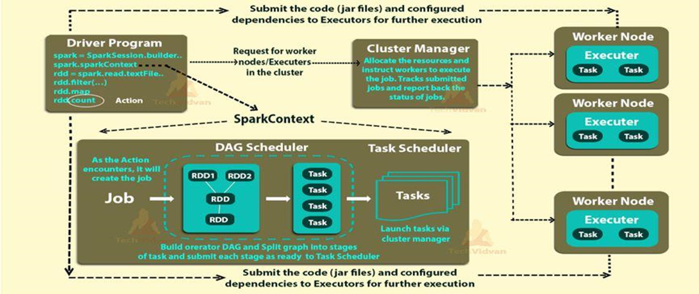
The architecture of an Apache Spark application is based on a distributed computing model that allows it to process large-scale data across multiple nodes in a cluster. Spark applications are designed to be fault-tolerant, scalable, and efficient. Here’s an overview of the key components and the flow of data in a typical Apache Spark application:

1. Driver Program:

• The Driver Program is the entry point of a Spark application. It runs on the master node and is responsible for creating the SparkContext, which is the entry point to any Spark functionality.
• The Driver Program defines the high-level control flow of the application, including tasks, stages, and dependencies between transformations and actions.

2. SparkContext (SC):

• SparkContext is the entry point to any Spark functionality. It establishes a connection to the cluster manager (e.g., YARN, Mesos, or Spark’s standalone cluster manager) to acquire resources for the application.
• The SparkContext coordinates with the Cluster Manager to allocate and manage executors across the worker nodes.

3. Cluster Manager:

• The Cluster Manager is responsible for managing the resources across the cluster, allocating tasks to workers, and ensuring fault tolerance.
• It can be YARN, Mesos, or Spark’s standalone cluster manager.

4. Worker Nodes:

• Worker Nodes are the machines in the cluster where actual data processing takes place.
• Each worker node hosts one or more executors, which are separate JVM processes responsible for executing tasks.

5. Executors:

• Executors are processes on the worker nodes responsible for executing individual tasks and storing data in memory or disk storage.
• They manage the data that is cached and reused across multiple Spark operations, reducing the need to read data from disk repeatedly.

6. Resilient Distributed Dataset (RDD):

• RDD is the fundamental data abstraction in Spark. It represents an immutable, fault-tolerant collection of objects that can be processed in parallel.
• RDDs are divided into partitions, and each partition is processed on a separate executor.

7. Transformations:

• Transformations are operations on RDDs that create new RDDs from existing ones. Examples include map, filter, reduceByKey, etc.
• Transformations are lazily evaluated, meaning they are not executed until an action is called.

8. Actions:

• Actions are operations that trigger the execution of transformations and return results to the Driver Program or write data to external storage.
• Examples of actions include collect, count, save, etc.
• Actions trigger the actual computation and materialize the RDD lineage.

9. Lineage Graph (DAG):

• Spark constructs a Directed Acyclic Graph (DAG) of the transformations (logical execution plan) and optimizes it before execution to minimize data shuffling and improve performance.

10. Data Sources and Sinks:

• Spark applications can read data from various sources (e.g., HDFS, S3, databases) and write data to external storage systems (e.g., HDFS, databases, file systems).

The architecture of Spark allows it to distribute data and computation across the cluster efficiently, providing fault tolerance, data locality, and high-performance data processing.

4. What is the maximum size of worker node you have used?

Storage 64 GB worker node.

Note – If you say more than that in interview garbage in and out problem occur so strict to max 64 GB.

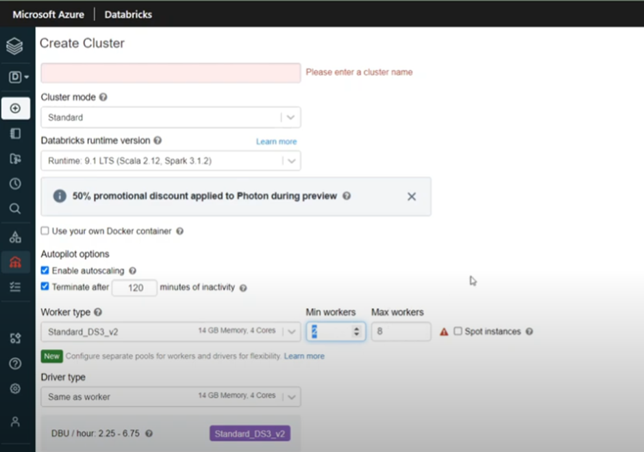
5. How do you choose cluster configuration in Databrics?

• For normal ETL/ELT work – Memory optimize
• Quick Dev test – General Purpose
• For Shuffle intensive work(e.g lot many join) – Storage optimize

6. What is the difference between repartition and coalesce?

Both repartition and coalesce are Spark transformations used to control the distribution of data across partitions in a DataFrame or an RDD (Resilient Distributed Dataset). They affect how data is physically stored and distributed across the nodes of a cluster.

In summary, the key differences are:

• repartition can increase or decrease the number of partitions and performs a full data shuffle, while coalesce only reduces the number of partitions and tries to minimize data movement.
• Use repartition when you need to achieve a specific number of partitions or evenly distribute data for better parallelism. Use coalesce when you want to reduce the number of partitions efficiently without triggering a full shuffle.

# For DataFrame repartition
df.repartition(numPartitions)
# For DataFrame coalesce
df.coalesce(numPartitions)

7. What is the drawback of coalesce?

The coalesce transformation in Spark is a powerful tool to reduce the number of partitions in a DataFrame or RDD without a full shuffle, which can be beneficial for certain use cases. However, it also has some drawbacks that you should be aware of:

Data Skew:

• When reducing the number of partitions with coalesce, Spark tries to minimize data movement and merges partitions into a smaller number of partitions. This approach can lead to data skew, where some partitions may end up with significantly more data than others.
• Data skew can negatively impact performance since a few partitions may become “hotspots” that are processed much slower than others, leading to inefficient resource utilization.

Uneven Data Distribution:

• Similar to data skew, coalesce can result in uneven data distribution across the reduced partitions. If the data has an uneven distribution or if certain keys have significantly more data than others, this can lead to suboptimal performance for subsequent operations like joins or aggregations.

Limited to Reduce Partitions:

• Unlike repartition, which allows you to increase or decrease the number of partitions, coalesce can only reduce the number of partitions. You cannot use coalesce to increase the number of partitions, which might be needed for certain operations that benefit from increased parallelism.

Less Parallelism:

• By reducing the number of partitions, you may reduce the level of parallelism in subsequent processing. This can lead to underutilization of resources, particularly if you have a large cluster with many available cores.

Optimal Partition Size:

• Choosing the right number of partitions for coalesce is crucial. If you set the number of partitions too low, you might end up with partitions that are too large to fit into memory, leading to performance issues.

8. If we have .gz file, how are they distributed in the spark

No, it will not be distributed, it will be single threaded.

9. What is the difference between “from pyspark.sql.type import *” and from pyspark.sql.types import xyz ?

Performance.

If we write from pyspark.sql.type import * every library under sql will get imported which will affect the performance.

10. What is the default partition size?

11. Have you worked on Databrics SQL? What is it all about?

Databrics SQL provides a simple experience for SQL users who wants to run quick ad-hoc queries on their data lake, create multiple visualization type to explore query result from different perspectives, and build and share dashboards.

12. What are the SQL endpoints? How are they different from cluster?

SQL endpoints in Databricks are secure entry points that allow users to execute SQL queries against their data. They provide a familiar SQL interface for querying and analyzing data stored in Databricks tables or external data sources like Delta Lake or Apache Spark tables.

Difference from cluster:

• A cluster in Databricks is a set of computing resources (e.g., virtual machines) used to run data processing and analytics workloads, such as Spark jobs and notebooks.
• SQL endpoints, on the other hand, are query interfaces specifically designed for executing SQL queries against data without the need to start a separate cluster.
• While clusters are general-purpose compute resources for various data processing tasks, SQL endpoints focus specifically on SQL query execution and can handle multiple concurrent queries efficiently.

13. What do you mean by interactive and job cluster?

Interactive Cluster: An interactive cluster in Databricks is designed for interactive data exploration and analysis. It provides a collaborative workspace where users can run notebooks and execute code interactively. Interactive clusters allow users to iteratively explore data, visualize results, and experiment with different analyses in a shared environment.

Job Cluster: A job cluster in Databricks is used for running batch jobs and automated data processing tasks. Unlike interactive clusters, job clusters are not continuously running and are launched on-demand to execute specific jobs at scheduled intervals or upon request. Job clusters are ideal for running ETL (Extract, Transform, Load) workflows, machine learning training, and other automated data processing tasks.

14. What is Auto scaling in databrics cluster?

• Auto Scaling in Databricks cluster automatically adjusts the cluster resources (number of worker nodes) based on workload demand, optimizing resource utilization and cost efficiency.
• Users can configure the Auto Scaling behaviour, setting minimum and maximum limits for the number of worker nodes and defining scaling policies based on metrics like CPU utilization or memory usage.

15. What is Managed and unmanaged tables in databrics?

In Databricks, managed and unmanaged tables are two different ways of organizing and managing data in the Databricks Delta Lake or Apache Spark table format:

Managed Tables:

• Managed tables, also known as Delta tables, are tables whose metadata and data files are managed and controlled by Databricks.
• When you create a managed table, Databricks handles the storage, organization, and cleanup of data files and metadata automatically.
• This means that when you delete a managed table, Databricks will also delete all the associated data files from storage.
• Managed tables are easy to work with since Databricks takes care of most of the underlying management tasks.

Unmanaged Tables:

• Unmanaged tables are tables where you have direct control over the data files, and Databricks does not manage the data or metadata.
• When you create an unmanaged table, you need to specify the data files’ location, and Databricks relies on you to handle file organization and cleanup.
• If you delete an unmanaged table, Databricks only removes the metadata, but the data files remain intact in the specified location.
• Unmanaged tables provide more control over the data, making them suitable for scenarios where you have existing data files in a specific location.

In summary, managed tables are automatically managed by Databricks, including data file storage and cleanup, while unmanaged tables require you to handle the data files’ management and organization manually.

16. How do you configure numbers of core in worker?

Generally, Number of cores = Numbers of partitions.

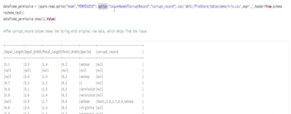
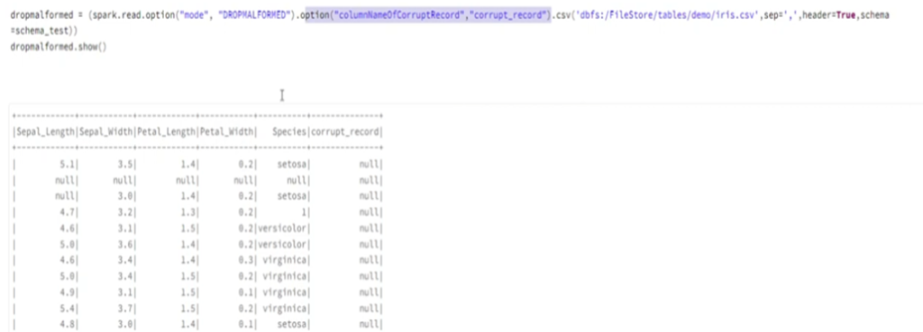
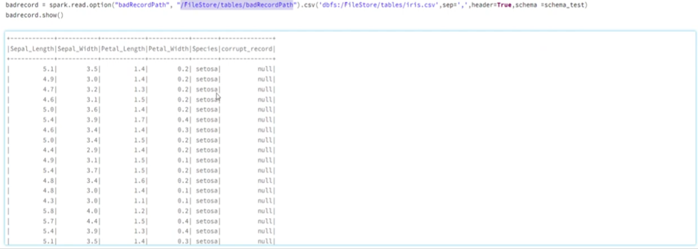
17. How do you handle BAD records in databrics?

There are two ways to handle errors in databrics:

MODE:

1. Permissive(Error value will be stored as null and entire error row will be saved as column)
2. Dropmalformed (Whole records that has error values will get drop off)
3. Failfast(When error is recognized execution stops)

BAD RECORD PATH (Redirect value to separate path)

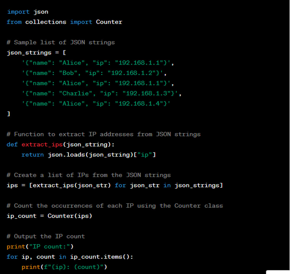
18. Given a list of json string, count the number of IP address, order of output does not matter?

To count the number of unique IP addresses from a list of JSON strings, you can follow these steps

1. Parse the JSON strings and extract the IP addresses.
2. Use a set to store the unique IP addresses.
3. Count the number of elements in the set, which will give you the count of unique IP addresses.

Here’s the Python code to achieve this:

Output:

19. What is difference between narrow and wide transformation?

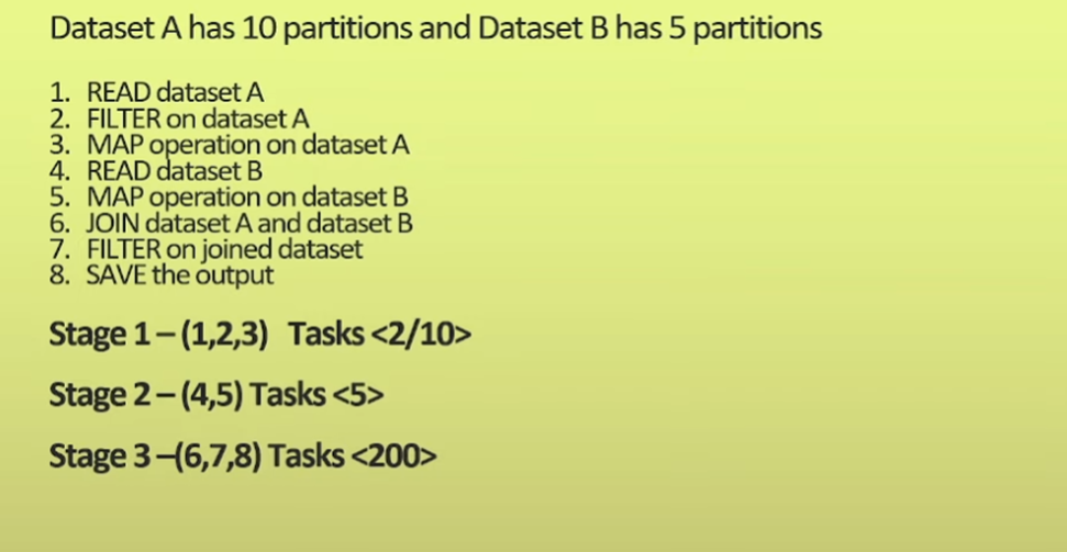
In Databricks (and Apache Spark), transformations are operations performed on a distributed dataset (RDD or DataFrame). These transformations are broadly classified into two categories: narrow transformations and wide transformations.

1. Narrow Transformations:

• Narrow transformations are transformations where each input partition contributes to at most one output partition.
• These transformations do not require data to be shuffled across the partitions, and they can be performed in parallel on each partition independently.
• Examples of narrow transformations include `map`, `filter`, and `union`.

2. Wide Transformations:

• Wide transformations are transformations where each input partition can contribute to multiple output partitions.
• These transformations require data to be shuffled and redistributed across the partitions, which involves a data exchange between the worker nodes.
• Wide transformations usually result in a stage boundary, which involves a physical data exchange and a shuffle operation.
• Examples of wide transformations include `groupBy`, `join`, and `sortByKey` (for RDDs).

The main difference between narrow and wide transformations lies in how they handle data distribution and shuffling. Narrow transformations can be executed efficiently in a parallel and distributed manner without the need for shuffling data between partitions. On the other hand, wide transformations require a data shuffle, which can be a more expensive operation as it involves network communication and data redistribution.

To optimize Spark job performance, it’s essential to minimize the usage of wide transformations and use them judiciously. When designing data processing pipelines, try to keep as many transformations as possible as narrow transformations to reduce data shuffling and improve execution efficiency.

20. What is shuffle? why shuffle occur? What causes the shuffle?

In the context of Apache Spark (and Databricks), a “shuffle” refers to the process of redistributing data across partitions in a distributed computing environment. Shuffle occurs when data needs to be rearranged to satisfy a specific operation, such as aggregations, joins, or sorting, where data from multiple partitions needs to be brought together to perform the operation effectively.

Shuffle occurs for the following reasons:

1. Data Reorganization for Operations:

• Certain operations, like grouping elements by a key in a `groupBy` or performing a `join` between two datasets, require data with the same keys to be brought together into the same partition to perform the operation.
• For example, when you perform a `groupBy` on a DataFrame or RDD based on a particular column, Spark needs to gather all the rows with the same key from various partitions and organize them together.

2. Data Skew:

• Data skew occurs when the distribution of data across partitions is uneven, causing some partitions to have significantly more data than others.
• In scenarios with data skew, a few partitions can become overloaded with data, leading to slower processing times for those partitions and suboptimal resource utilization.
• To handle data skew, Spark may need to redistribute data through shuffle to achieve a more balanced data distribution across partitions.

3. Performance Optimization:

• In some cases, shuffle can be used to optimize performance by co-locating related data on the same partitions, reducing the amount of data exchange during certain operations.
• For example, Spark can leverage shuffle to bring together data that will be accessed together, reducing the need to read data from various partitions separately.

It’s essential to be aware of the cost of shuffle operations since they involve data movement across the network, which can be expensive in terms of computation and time. Minimizing shuffle whenever possible is a key performance consideration when designing and optimizing Apache Spark or Databricks jobs. Proper partitioning of data and careful selection of appropriate operations can help reduce the frequency and impact of shuffling.

21. What is difference between sortBy and OrderBy?

We can use either sort() or Orderby() built in function to sort a particular dataframe in a ascending or descending order over at least one column.

Sort()

Sort() method will sort() the records in each partition and then return the final output which means that the order of the output data is not guaranteed because data is ordered on partition level but your data frame may have thousands of partitions distributed across the cluster.

Since the data is not collected into a single executor the sort() method is efficient thus more suitable  when sorting is not critical for your use case.

Orderby()

Unlike Sort(), the orderBy() function guarantee a total order in the output. This happen because the data will be collected into a single executor in order to be sorted.

This means that orderBy() is more inefficient compared to sort()

22. What is difference between map and map partition?

map()

map is a transformation that applies a function to each element of the RDD or DataFrame, processing the elements one at a time. whatever transformation you mentation on the data. It has a one-to-one mapping between input and output elements.

mapPartitions()

mapPartitions is a transformation that applies a function to each partition of the RDD or DataFrame, processing multiple elements within each partition at once. It has a one-to-many mapping between input partitions and output partitions.

In summary, map processes data element-wise, while mapPartitions processes data partition-wise, which can lead to more efficient data processing when dealing with expensive operations or when you need to maintain some state across multiple elements within a partition.

23. What is lazy evaluation in spark?

Lazy evaluation in Spark refers to the evaluation strategy where transformations on RDDs (Resilient Distributed Datasets) or DataFrames are not executed immediately when called. Instead, Spark builds up a logical execution plan (DAG – Directed Acyclic Graph) representing the sequence of transformations. The actual execution is deferred until an action is called.

Key points about lazy evaluation in Spark:

Transformations are Deferred:

When you apply a transformation on an RDD or DataFrame (e.g., `map`, `filter`, `groupBy`, etc.), Spark does not perform the actual computation right away. Instead, it records the transformation in the execution plan.

Logical Execution Plan (DAG):

Spark builds a directed acyclic graph (DAG) that represents the series of transformations in the order they were applied. Each node in the DAG represents a transformation, and the edges represent data dependencies.

Efficient Optimization:

Since Spark has access to the entire transformation sequence before executing any action, it can optimize the execution plan for performance, by combining and reordering transformations to reduce data shuffling and improve parallelism.

Lazy Execution with Actions:

Spark only performs the actual computation when an action is called (e.g., `collect`, `count`, `save`, etc.). Actions trigger the execution of the entire DAG of transformations, starting from the original RDD or DataFrame.

Benefits of lazy evaluation:

• It allows Spark to optimize the execution plan before actually running the job, leading to more efficient data processing.
• Lazy evaluation reduces unnecessary computation and data shuffling, as Spark can skip intermediate transformations that are not needed to compute the final result.
• It provides an opportunity for developers to chain multiple transformations together before triggering the actual computation, which can lead to more concise and modular code.

Overall, lazy evaluation is a fundamental optimization technique in Spark that improves performance by deferring the execution of transformations until the results are required.

24. What are the different levels of persistence in spark?

In Apache Spark, persistence (also known as caching) is a technique to store intermediate or final computation results in memory or disk. By persisting data, Spark can reuse it across multiple Spark operations without re-computing it from the original data source. This can significantly improve the performance of iterative algorithms or when the same data is accessed multiple times.

There are different levels of persistence available in Spark:

1. MEMORY_ONLY (or MEMORY_ONLY_SER):

• This is the simplest level of persistence, where the RDD or DataFrame is stored in memory as deserialized Java objects (MEMORY_ONLY) or serialized bytes (MEMORY_ONLY_SER).
• MEMORY_ONLY is suitable when the data fits comfortably in memory and can be quickly accessed without deserialization overhead.
• MEMORY_ONLY_SER is useful when the data size is larger than the available memory, as it saves memory space by keeping the data in a serialized format.

2. MEMORY_AND_DISK:

• In this level of persistence, if an RDD or DataFrame does not fit entirely in memory, Spark spills the excess partitions to disk while keeping the remaining partitions in memory.
• MEMORY_AND_DISK provides a balance between in-memory access speed and disk space utilization. However, accessing data from disk is slower than accessing it from memory, so it may lead to performance degradation for frequently accessed data that spills to disk.

3. MEMORY_AND_DISK_SER:

• Similar to MEMORY_AND_DISK, but it stores data in serialized format to save memory space.
• MEMORY_AND_DISK_SER can be beneficial when the dataset is large and cannot fit entirely in memory.

4. DISK_ONLY:

• In this level of persistence, data is stored only on disk and not kept in memory.
• DISK_ONLY is suitable when memory is limited, and the data size is much larger than the available memory.
• Accessing data from disk is slower than accessing it from memory, so performance might be affected.

5. OFF_HEAP:

• This is an experimental feature in Spark that stores data off-heap (outside the JVM heap space).
• OFF_HEAP is useful for very large datasets that require a significant amount of memory, as it can help avoid Java garbage collection overhead.

Each persistence level offers different trade-offs between memory utilization and access speed. The choice of persistence level depends on factors like the size of data, available memory, and the frequency of data access in your Spark application. Properly selecting the persistence level can greatly impact the overall performance and efficiency of Spark jobs.

Import org.apache.spark.storage.storagelevel
Val rdd2 = rdd.persist(StorageLevel.MEMORY_ONLY)

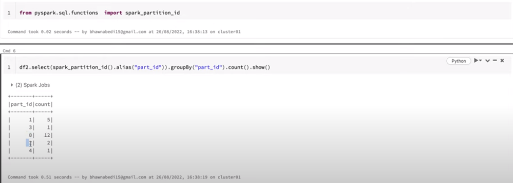
25. How to check data skewness of how many rows present in each partition?

26. What are the different planes in Databrics?

In cloud computing and distributed systems, the concept of “planes” is used to categorize different aspects of the system’s architecture and management. The three main planes are:

Data Plane:

• The Data Plane is responsible for handling and processing the actual user data and performing the intended operations on the data.
• In Databricks, the Data Plane is where data processing tasks take place, such as executing Spark jobs, running notebooks, and performing data transformations.

Control Plane:

• The Control Plane is responsible for managing and coordinating the overall system’s operation and behavior.
• In Databricks, the Control Plane manages the cluster lifecycle, monitors resource allocation, schedules jobs, and handles administrative tasks such as authentication, access control, and cluster management.

Management Plane:

• The Management Plane provides tools and interfaces for users and administrators to configure, monitor, and manage the system and its components.
• In Databricks, the Management Plane includes the Databricks Workspace, which provides a collaborative environment for managing notebooks, libraries, dashboards, and other resources.

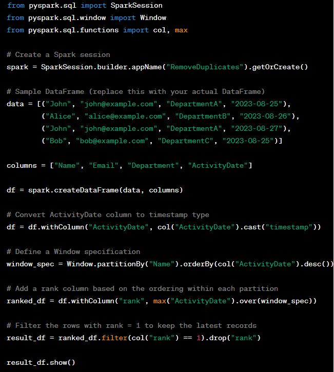
Each plane plays a crucial role in the operation and management of cloud-based distributed systems like Databricks, helping to separate concerns and provide a clear and organized way to design and manage complex systems.

27. How to drop duplicate from following dataframe?

STATION_ID	DATE_CHANGED  STATION_ID
1	6/7/2006 6:00
1	9/26/2000 6:00
2	7/29/2005 6:00
2	6/6/2001 6:00
4	6/8/2001 6:00
4	11/25/2003 7:00
7	6/12/2001 6:00
8	6/4/2001 6:00
8	4/3/2017 18:36

df.sort_values('DATE_CHANGED').drop_duplicates('STATION_ID',keep='last')

28. How to improve performance of a notebook in databrics?

To improve notebook performance in Databricks, you can follow these best practices and optimization techniques:

1. Cluster Configuration: Use an appropriately sized cluster based on your workload. Scaling up the cluster can significantly improve performance, especially for resource-intensive tasks. Databricks provides various cluster types with different CPU, memory, and GPU configurations. You can monitor cluster performance to identify bottlenecks.

 2. Autoscaling: Enable autoscaling to automatically adjust the number of workers based on the workload. This helps optimize resource allocation and reduce costs during idle periods.

 3. Caching and Persistence: Utilize caching and persistence to store intermediate results or dataframes that are frequently accessed. This can speed up subsequent operations by avoiding redundant computations.

 4. Optimize Data Format: Choose appropriate data formats to store and read data. For example, using Parquet format for storage is more efficient than using CSV or JSON due to its columnar storage and compression capabilities.

5. Limit Data Shuffling: Minimize data shuffling as it can be a resource-intensive operation. Data shuffling occurs when the data needs to be redistributed across partitions, and it can impact performance significantly.

 6. Tune Spark Configurations: Adjust Spark configurations like `spark.sql.shuffle.partitions`, `spark.executor.memory`, and `spark.driver.memory` to optimize performance based on your specific workload and data size.

7. Use Delta Lake: If possible, leverage Delta Lake for transactional and versioned data storage. It offers significant performance improvements for analytics workloads.

 8. Spark UI Optimization: Use the Spark UI to monitor job progress, identify performance bottlenecks, and optimize query plans. Look for stages with long execution times or high shuffle data, and try to optimize them.

 9. Use Databricks Runtime: Databricks Runtime is optimized by default and includes various performance improvements. Always use the latest stable version for the best performance and new features.

 10. Notebook Code Optimization: Review and optimize your notebook code regularly. Avoid unnecessary data transformations and use efficient Spark APIs and DataFrame operations when possible.

 11. Resource Management: Be mindful of resource utilization in notebooks. Avoid running multiple long-running notebooks simultaneously to prevent resource contention.

 12. Data Pruning: For large datasets, consider pruning the data to limit the amount of data processed, especially if you only need a specific time range or subset of data.13. External Data Cache: Use the Databricks External Data Cache to cache data across multiple notebooks or clusters, reducing data transfer time and computation overhead.

Remember that the effectiveness of these optimizations depends on your specific use case and data, so it’s essential to monitor and fine-tune your configurations regularly to achieve the best performance.

29. How to pass parameter though parent notebook in the child notebook?

In Databricks, you can pass parameters from a parent notebook to a child notebook using the dbutils.notebook.run function. This function allows you to call a child notebook and pass parameters as input to the child notebook. Here’s a step-by-step guide on how to do this.

Step 1: Define the Parent Notebook:

In the parent notebook, you can define the parameters you want to pass to the child notebook and then call the child notebook using the dbutils.notebook.run function.

# Parent Notebook

param1 = "value1"
param2 = 42

dbutils.notebook.run("ChildNotebook", 0, {"param1": param1, "param2": param2})

Step 2: Access Parameters in the Child Notebook:

In the child notebook, you can access the parameters passed from the parent notebook using the dbutils.widgets module. You need to define widgets with the same names as the parameters used in the parent notebook.

# ChildNotebook

param1 = dbutils.widgets.get("param1")
param2 = dbutils.widgets.get("param2")

print("Received parameters in child notebook:")
print("param1:", param1)
print("param2:", param2)

By using the dbutils.widgets.get function with the same name as the parameter, you can retrieve the values passed from the parent notebook.

30. What are the dbutils function available in databrics?

In Databricks, the `dbutils` module provides utility functions that help you interact with the Databricks environment, access files, manage libraries, and more. These functions are designed to simplify common tasks when working with Databricks notebooks and clusters. Here are some of the commonly used `dbutils` functions available in Databricks:

1. File System Operations:

•    dbutils.fs.ls(path): List files in a directory.
•    dbutils.fs.cp(source, destination): Copy a file or directory.
•    dbutils.fs.mv(source, destination): Move or rename a file or directory.
•    dbutils.fs.rm(path, recurse=True): Remove a file or directory.
•    dbutils.fs.mkdirs(path): Create directories recursively.

2. Notebook Utilities:

   – `dbutils.notebook.run(notebook_path, timeout_seconds, arguments)`: Run a different notebook and pass parameters.
   – `dbutils.notebook.exit(result)`: Stop execution of the current notebook and return a result.

3. Widgets:
   – dbutils.widgets.text(name, defaultValue): Create a text widget.
   – dbutils.widgets.get(name): Get the value of a widget.
   – dbutils.widgets.dropdown (name, defaultValue, choices): Create a dropdown widget.
   – dbutils.widgets.combobox (name, defaultValue, choices): Create a combo box widget.
   – dbutils.widgets.multiselect (name, defaultValue, choices): Create a multiselect widget.

 4. Library Management:
   – dbutils.library.install (pypi_package): Install a PyPI package as a library.
   – dbutils.library.restartPython(): Restart the Python interpreter to apply library changes.
   – dbutils.library.remove (library_path): Remove a library.

 5. Secret Management:
   – dbutils.secrets.get(scope, key): Retrieve a secret from the Databricks Secret Manager.

 6. Azure Blob Storage Utilities:
   – dbutils.fs.mount(source, mount_point): Mount an Azure Blob Storage container.
   – dbutils.fs.unmount(mount_point): Unmount an Azure Blob Storage container.

31. What is broadcast join?

In Databricks, a broadcast join is a type of join operation used in Spark SQL that optimizes the performance of joining a small DataFrame (or table) with a larger DataFrame (or table). It is based on the concept of broadcasting the smaller DataFrame to all the nodes of the cluster, allowing each node to perform the join locally without shuffling the data. This approach is beneficial when one of the DataFrames is small enough to fit in memory and the other DataFrame is significantly larger.

When performing a broadcast join, Spark automatically broadcasts the smaller DataFrame to all the worker nodes in the cluster, making it available in memory. Then, the worker nodes use this broadcasted copy to perform the join locally with their respective partitions of the larger DataFrame. By doing so, Spark can avoid costly shuffling operations, which can lead to significant performance improvements.

To leverage the benefits of a broadcast join in Spark SQL, you can explicitly hint the optimizer to use it for a specific join by using the BROADCAST keyword. For example:

By adding the /*+ BROADCAST(small_df) */ hint to the SQL query, you inform Spark to use a broadcast join for the specified small_df DataFrame.

32. What is struct function?

In Databricks, the struct function is a Spark SQL function used to create a new struct column by combining multiple columns together. A struct column is similar to a struct or namedtuple in programming languages, allowing you to group multiple values together into a single column. This is especially useful when you want to create complex data types or nest multiple fields within a single DataFrame column.

The struct function takes multiple column expressions as arguments and returns a new column containing the combined values as a struct. Each input column becomes a field within the resulting struct column. The struct columns can then be used like any other DataFrame column, allowing you to access nested data in a structured manner.

Here’s the basic syntax of the struct function:

• column1, column2, …, columnN: The input columns that you want to combine into the struct column.

Here’s a practical example of using the struct function:

Output look like this:

33. What is explode function does?

In Databricks, the explode function is a Spark SQL function used to transform an array or map column into multiple rows, effectively “exploding” the elements of the array or map into separate rows. This is particularly useful when you have data with nested arrays or maps, and you want to flatten the structure to perform operations on individual elements.

The explode function works on columns that contain arrays or maps and produces a new DataFrame with each element of the array or map expanded into separate rows. For arrays, each element of the array becomes a separate row, and for maps, the key-value pairs of the map become separate rows.

Here’s the basic syntax of the explode function:

• column: The column containing the array or map that you want to explode.
• alias: An optional alias to give a name to the resulting column after the explosion.

Let’s look at a practical example using the explode function:

The output will look like:

As you can see, the fruits array column is exploded into separate rows, where each fruit from the array becomes an individual row in the resulting DataFrame.

The explode function is a powerful tool when working with nested data structures, and it allows you to perform operations on individual elements within arrays or maps efficiently in Databricks. It can be combined with other Spark SQL functions to perform complex data manipulations on nested data.

34. Is it possible to combine Databricks and Azure Notebooks?

They operate similarly, but data transfer to the cluster requires manual coding. This Integration is now easily possible thanks to Databricks Connect. On behalf of Jupyter, Databricks makes a number of improvements that are specific to Databricks.

35. What exactly does caching entail?

Temporary holding is referred to as the cache. The process of temporarily storing information is referred to as caching. You’ll save time and lessen the load on the server when you come back to a frequently visited website because the browser will retrieve the data from the cache rather than from the server.

36. What are the different types of caching are there?

There are four types of caching that stand out:

• Information caching
• Web page caching
• Widespread caching
• Output or application caching.

37. Should you ever remove and clean up any leftover Data Frames?

Cleaning Frames is not necessary unless you use cache(), which will use a lot of network bandwidth. You should probably clean up any large datasets that are being cached but aren’t being used.

38. What different ETL operations does Azure Databricks carry out on data?

The various ETL processes carried out on data in Azure Databricks are listed below:

• The data is converted from Databricks to the data warehouse.
• Bold storage is used to load the data.
• Data is temporarily stored using bold storage

39. Does Azure Key Vault work well as a substitute for Secret Scopes?

That is certainly doable. However, some setup is necessary. The preferred approach is this. Instead of changing the defined secret, start creating a scoped password that Azure Key Vault will backup if the data in secret needs to be changed.

40. How should Databricks code be handled when using TFS or Git for collaborative projects?

TFS is not supported, to start. Your only choices are dispersed Git repository systems and Git. Although it would be ideal to integrate Databricks with the Git directory of notebooks, it works much like a different project clone. Making a notebook, trying to commit it to version control, and afterwards updating it are the first steps.

41. Does Databricks have to be run on a public cloud like AWS or Azure, or can it also run on cloud infrastructure?

This is not true. The only options you have right now are AWS and Azure. But Databricks uses Spark, which is open-source. Although you could build your own cluster and run it in a private cloud, you’d be giving up access to Databricks’ robust features and administration.

42. How is a Databricks personal access token created?

• On the Databricks desktop, click the “user profile” icon in the top right corner.
• Choosing “User setting.”
• Activate the “Access Tokens” tab.
• A “Generate New Token” button will then show up. Just click it.

43. Is code reuse possible in the Azure notebook?

We should import the code first from Azure notebook into our notebook so that we can reuse it. There are two ways we can import it.

• We must first create a component for the code if it is located on a different workstation before integrating it into the module.
• We can import and use the code right away if it is on the same workstation.

44. What is a Databricks cluster?

The settings and computing power that make up a Databricks cluster allow us to perform statistical science, big data, and powerful analytic tasks like production ETL, workflows, deep learning, and stream processing.

45. Is databrics provide database services, if no then where it saves the delta table?

Azure Databricks does not directly provide traditional database services like SQL Server or Azure SQL Database. Instead, it is an Apache Spark-based analytics platform designed to process and analyze big data workloads. However, it can work with various data sources and databases to perform data processing and analytics tasks.

One of the popular data storage options in Azure Databricks is Delta Lake, which is an open-source storage layer that brings ACID (Atomicity, Consistency, Isolation, Durability) transactions to data lakes. Delta Lake provides some database-like functionalities on top of cloud storage systems like Azure Data Lake Storage or Azure Blob Storage.

When you save a Delta table in Azure Databricks, the data is typically stored in your specified cloud storage (e.g., Azure Data Lake Storage or Azure Blob Storage). Delta Lake keeps track of the changes made to the data, allowing for versioning and transactional capabilities.

46. Is Databricks only available in the cloud and does not have an on-premises option?

Yes. Databricks’ foundational software, Apache Spark, was made available as an on-premises solution, allowing internal engineers to manage both the data and the application locally. Users who access Databricks with data on local servers will encounter network problems because it is a cloud-native application. The on-premises choices for Databricks are also weighed against workflow inefficiencies and inconsistent data.

47. In Parameter what does it mean by inferSchema as True

In the context of data processing frameworks like Apache Spark and PySpark (used in Azure Databricks), the inferSchema parameter is used when reading data from external sources like CSV, JSON, Parquet, etc. It is a configuration option that determines whether Spark should automatically infer the data types of the columns in the DataFrame based on the data content.

When inferSchema is set to True, Spark will automatically examine a sample of the data to infer the data types for each column. This process involves analyzing the data values in each column and making educated guesses about the appropriate data types. For example, if a column predominantly contains numeric values, Spark might infer it as an integer or a double data type. Similarly, if a column primarily contains strings, it might infer it as a string data type.

Setting inferSchema to True can be convenient and save time, especially when working with large datasets with many columns. Spark’s ability to automatically infer data types allows you to read data without explicitly specifying the schema, making the code shorter and more flexible.

However, it’s essential to be cautious when using inferSchema, as it relies on a sample of the data and might not always make accurate decisions, especially when the data is sparse or there are outliers. In such cases, it’s recommended to provide an explicit schema to ensure the correct data types are used.

48. What are the difference between Auto Loader vs COPY INTO?

Auto Loader:

Auto Loader incrementally and efficiently processes new data files as they arrive in cloud storage without any additional setup. Auto Loader provides a new Structured Streaming source called cloudFiles. Given an input directory path on the cloud file storage, the cloudFiles source automatically processes new files as they arrive, with the option of also processing existing files in that directory.

When to use Auto Loader instead of the COPY INTO?

• If you’re going to ingest files in the order of thousands, you can use COPY INTO. If you are expecting files in the order of millions or more over time, use Auto Loader. Auto Loader requires fewer total operations to discover files compared to COPY INTO and can split the processing into multiple batches, meaning that Auto Loader is less expensive and more efficient at scale.
• If your data schema is going to evolve frequently, Auto Loader provides better primitives around schema inference and evolution. See Configure schema inference and evolution in Auto Loader for more details.
• Loading a subset of re-uploaded files can be a bit easier to manage with COPY INTO. With Auto Loader, it’s harder to reprocess a select subset of files. However, you can use COPY INTO to reload the subset of files while an Auto Loader stream is running simultaneously.

spark.readStream.format("cloudfiles") # Returns a stream data source, reads data as   it arrives based on the trigger.

.option("cloudfiles.format","csv") # Format of the incoming files
.option("cloudfiles.schemalocation", "dbfs:/location/checkpoint/")  The location to store the inferred schema and subsequent changes

.load(data_source)
.writeStream.option("checkpointlocation","dbfs:/location/checkpoint/") # The location of the stream’s checkpoint

.option("mergeSchema", "true") # Infer the schema across multiple files and to merge the schema of each file. Enabled by default for Auto Loader when inferring the schema.

.table(table_name)) # target table

49. How to do partition data in the databrics?

Partitioning data in Databricks, or any other data processing platform, can greatly improve query performance and overall data organization. Partitioning involves dividing your data into smaller, more manageable parts based on specific criteria, such as a particular column’s values. This helps reduce the amount of data that needs to be scanned when executing queries, leading to faster query execution times. Here’s how you can partition data in Databricks:

1. Choose a Partition Column: Select a column in your dataset that you want to use for partitioning. Common choices are date columns, country codes, or any other attribute that can be used to logically group your data.

2. Organize Data: Arrange your data in the storage system (like a data lake) in a way that reflects the partitioning scheme you’ve chosen. This usually involves creating subdirectories for each partition, where the name of the subdirectory corresponds to the partition key’s value. For example, if you’re partitioning by year and month, your directory structure might look like:

3. Write Partitioned Data: When writing data into Databricks, make sure to specify the partition column and value appropriately. Databricks has integrations with various data sources like Parquet, Delta Lake, and more, which support partitioning.

For example, if you’re using Apache Spark to write partitioned Parquet data, you can do something like this:

4. Querying Partitioned Data: When querying partitioned data, Databricks and Spark will automatically take advantage of the partitioning scheme to optimize query performance. You can filter your queries based on the partition column, and Spark will only scan the relevant partitions, reducing the amount of data scanned.

50. How to rename a column name in dataframe?

51. If we have an employee data frame and we want to add 1000 to those employee’s salary who have a more than 10,000 salary how to do that?

You can achieve this using PySpark by applying a transformation to the DataFrame to update the salary values based on a condition. Here’s a sample code to add 1000 to the salary of employees who have a salary greater than 10,000:

Update using multiple conditions.

52. What is surrogate key in database concept?

A surrogate key is a unique identifier that is added to a database table to serve as a primary key. Unlike natural keys, which are based on existing data attributes (such as names, dates, or other real-world information), surrogate keys are typically artificially created and have no inherent meaning. They are used primarily to improve the efficiency and performance of database operations.

Surrogate keys offer several benefits:

1. Uniqueness: Surrogate keys are generated in a way that ensures their uniqueness across the entire table. This eliminates the risk of duplicate entries that might occur with natural keys.

2. Stability: Since surrogate keys are not based on changing attributes like names or addresses, they remain stable over time. This makes them ideal for linking data and maintaining relationships even when other attributes change.

3. Performance: Surrogate keys can improve database performance by making indexes and joins more efficient. They tend to be shorter than meaningful attributes, leading to faster data retrieval and better query performance.

4. Data Privacy: Surrogate keys help maintain data privacy by not exposing sensitive or personal information in the key itself. This can be important for compliance with data protection regulations.

5. Simplifying Joins: When tables are linked through relationships, using surrogate keys can simplify the process of joining tables, as the keys are consistent and predictable.

6. Data Warehousing: In data warehousing scenarios, surrogate keys are often used to create fact and dimension tables, facilitating efficient reporting and analysis.

An example of a surrogate key might be an auto-incrementing integer that is assigned to each new record added to a table. This key is unique and has no inherent meaning, making it an ideal primary key for efficient database operations.

It’s worth noting that while surrogate keys offer various advantages, there are cases where natural keys (based on meaningful attributes) might be more appropriate, especially when the data itself carries important semantic meaning. The choice between surrogate and natural keys depends on the specific requirements of the database schema and the overall data model.

53. If I have a dataframe called student where I have Name, email, department and activity date columns. email column has some duplicate how to remove duplicate name but want to keep the latest records using window function?

In this code, a window specification is defined partitioned by the “Name” column and ordered by the “ActivityDate” in descending order. The max("ActivityDate").over(window_spec) calculates the maximum activity date within each partition (each name). Then, we filter the rows where the rank is equal to 1, which corresponds to the latest records within each partition.

54. What is Delta Table Versioning ? give an example.

Delta table versioning in Databricks is a feature of Delta Lake, an open-source storage layer that brings ACID (Atomicity, Consistency, Isolation, Durability) transactions to Apache Spark and big data workloads. Delta Lake provides the ability to perform time travel operations, which allows users to query data as it existed at a specific point in time. This is enabled by Delta table versioning.

Let’s say you have a Delta table named ‘sales_data‘, and you want to view the state of the table as it was at version 5 or as it was at a specific timestamp:

55. Is there a hard limit on the maximum number of versions you can retrieve data from? How to Configure Retention Policies?

In Delta Lake, there isn’t a hard limit on the maximum number of versions you can retrieve data from. However, practical limits are imposed by storage costs, performance considerations, and retention policies.

Factors Influencing Version Retention:

1. Storage Costs:
   • Each version of a Delta table requires storage space. If you retain many versions, the storage cost will increase accordingly.
2. Performance:
   • As the number of versions increases, certain operations (like querying historical data) might become slower due to the increased size of the transaction log.
3. Retention Policies:
   • You can configure Delta Lake to automatically clean up old versions based on a defined retention policy. This helps in managing storage costs and maintaining performance.

Configuring Retention Policies:

Delta Lake provides a vacuum command to remove old data files and log files, which helps in managing the number of versions:

This command will retain the last 168 hours (7 days) of versions. You can adjust the retention period based on your requirements.

How do you assess the statistical significance of an insight?

We need to perform hypothesis testing to determine statistical significance. Will take following steps.

• First will define null hypothesis and alternate hypothesis
• We will calculate p- value
• Last, we would set the level of the significance (alpha) and if the p-value is less than the alpha, you would reject the null — in other words, the result is statistically significant.

What is the Central Limit Theorem and why is it important?

• Central limit theorem is very important concept in stats. It states that no matter the underlying distribution of the data set, the sampling distribution would be equal to the mean of original distribution and variance would be n times smaller, where n is the size of sample
• The central limit theorem (CLT) states that the distribution of sample means approximates a normal distribution as the sample size gets larger.
• Sample sizes equal to or greater than 30 are considered sufficient for the CLT to hold.
• A key aspect of CLT is that the average of the sample means and standard deviations will equal the population mean and standard deviation.

Example-

Suppose that we are interested in estimating the average height among all people. Collecting data for every person in the world is impossible. While we can’t obtain a height measurement from everyone in the population, we can still sample some people. The question now becomes, what can we say about the average height of the entire population given a single sample. The Central Limit Theorem addresses this question exactly.”

What is sampling? How many sampling methods do you know?

Data sampling is a statistical analysis technique used to select, manipulate and analyse a subset of data points to identify patterns and trends in the larger data set. It enables data scientists and other data analysts to work with a small, manageable amount of data about a statistical population to build and run analytical models more quickly, while still producing accurate findings.

• Simple random sampling: Software is used to randomly select subjects from the whole population.
• Stratified sampling: Subsets of the data sets or population are created based on a common factor, and samples are randomly collected from each subgroup.
• Cluster sampling: The larger data set is divided into subsets (clusters) based on a defined factor, then a random sampling of clusters is analyzed.
• Multistage sampling: A more complicated form of cluster sampling, this method also involves dividing the larger population into a number of clusters. Second-stage clusters are then broken out based on a secondary factor, and those clusters are then sampled and analyzed. This staging could continue as multiple subsets are identified, clustered and analyzed.
• Systematic sampling: A sample is created by setting an interval at which to extract data from the larger population — for example, selecting every 10th row in a spreadsheet of 200 items to create a sample size of 20 rows to analyze.

Explain selection bias (with regard to a dataset, not variable selection). Why is it important? How can data management procedures such as missing data handling make it worse?

Selection bias is the phenomenon of selecting individuals, groups or data for analysis in such a way that proper randomization is not achieved, ultimately resulting in a sample that is not representative of the population.

Types of selection bias include:

• sampling bias: a biased sample caused by non-random sampling
• time interval: selecting a specific time frame that supports the desired conclusion. e.g. conducting a sales analysis near Christmas.
• attrition: attrition bias is similar to survivorship bias, where only those that ‘survived’ a long process are included in an analysis, or failure bias, where those that ‘failed’ are only included
• observer selection: related to the Anthropic principle, which is a philosophical consideration that any data we collect about the universe is filtered by the fact that, in order for it to be observable, it must be compatible with the conscious and sapient life that observes it. 

Handling missing data can make selection bias worse because different methods impact the data in different ways. For example, if you replace null values with the mean of the data, you adding bias in the sense that you’re assuming that the data is not as spread out as it might actually be.

What is the difference between type I vs type II error?

Anytime we make a decision using statistics there are four possible outcomes, with two representing correct decisions and two representing errors.

Type – I Error:

A type 1 error is also known as a false positive and occurs when a researcher incorrectly rejects a true null hypothesis. This means that your report that your findings are significant when in fact they have occurred by chance.

The probability of making a type I error is represented by your alpha level (α), which is the p-value. A p-value of 0.05 indicates that you are willing to accept a 5% chance that you are wrong when you reject the null hypothesis

Type – II Error:

A type II error is also known as a false negative and occurs when a researcher fails to reject a null hypothesis which is really false. Here a researcher concludes there is not a significant effect, when actually there really is.

The probability of making a type II error is called Beta (β), and this is related to the power of the statistical test (power = 1- β). You can decrease your risk of committing a type II error by ensuring your test has enough power.

What are the four main things we should know before studying data analysis?

Following are the key point that we should know:

• Descriptive statistics
• Inferential statistics
• Distributions (normal distribution / sampling distribution)
• Hypothesis testing

What is the difference between inferential statistics and descriptive statistics?

Descriptive Analysis – It uses the data to provide description of the population either through numerical calculations or graph or tables.

Inferential statistics – Provides information of a sample and we need to inferential statistics to reach to a conclusion about the population.

How to calculate range and interquartile range?

IQR = Q3 – Q1

Where, Q3 is the third quartile (75 percentile) 

Where, Q1 is the first quartile (25 percentile)

What is the benefit of using box plot?

A box plot, also known as a box and whisker plot, is a type of graph that displays a summary of a large amount of data in five numbers. These numbers include the median, upper quartile, lower quartile, minimum and maximum data values.

Following are the advantages of Box-plot:

• Handle Large data easily – Due to the five-number data summary, a box plot can handle and present a summary of a large amount of data. Organizing data in a box plot by using five key concepts is an efficient way of dealing with large data too unmanageable for other graphs, such as line plots or stem and leaf plots.
• A box plot shows only a simple summary of the distribution of results, so that it you can quickly view it and compare it with other data.
• A box plot is a highly visually effective way of viewing a clear summary of one or more sets of data. 
• A box plot is one of very few statistical graph methods that show outliers. Any results of data that fall outside of the minimum and maximum values known as outliers are easy to determine on a box plot graph.

What is the meaning of standard deviation?

It represents how far are the data points from the mean

(σ) = √(∑(x-µ)² / n)

Variance is the square of standard deviation

What is left skewed distribution and right skewed distribution?

Left skewed

• The left tail is longer than the right side
  • Mean < median < mode

Right skewed

• The right tail is longer than the left side
  • Mode < median < mean

What does symmetric distribution mean?

The part of the distribution that is on the left side of the median is same as the part of the distribution that is on the right side of the median

Few examples are – uniform distribution, binomial distribution, normal distribution

What is the relationship between mean and median in normal distribution?

In the normal distribution mean is equal to median

What does it mean by bell curve distribution and Gaussian distribution?

Normal distribution is called bell curve distribution / Gaussian distribution.It is called bell curve because it has the shape of a bell.It is called Gaussian distribution as it is named after Carl Gauss.

How to convert normal distribution to standard normal distribution?

Standardized normal distribution has mean = 0 and standard deviation = 1. To convert normal distribution to standard normal distribution we can use the formula

X (standardized) = (x-µ) / σ

What is an outlier? What can I do with outlier?

An outlier is an abnormal value (It is at an abnormal distance from rest of the data points). 

Following thing we can do with outliers

Remove outlier

• When we know the data-point is wrong (negative age of a person)
  • When we have lots of data
  • We should provide two analyses. One with outliers and another without outliers.

Keep outlier

• When there are lot of outliers (skewed data)
  • When results are critical
  • When outliers have meaning (fraud data)

What is the difference between population parameters and sample statistics?

Population parameters are:

• Mean = µ
  • Standard deviation = σ

Sample statistics are:

• Mean = x (bar)
  • Standard deviation = s

How to find the mean length of all fishes in the sea?

Define the confidence level (most common is 95%). Take a sample of fishes from the sea (to get better results the number of fishes > 30). Calculate the mean length and standard deviation of the lengths. Calculate t-statistics. Get the confidence interval in which the mean length of all the fishes should be.

What are the effects of the width of confidence interval?

• Confidence interval is used for decision making
• As the confidence level increases the width of the confidence interval also increases
• As the width of the confidence interval increases, we tend to get useless information also.

Mention the relationship between standard error and margin of error?

As the standard error increases the margin of error also increases.

What is p-value and what does it signify?

The p-value reflects the strength of evidence against the null hypothesis. p-value is defined as the probability that the data would be at least as extreme as those observed, if the null hypothesis were true.

• P- Value > 0.05 denotes weak evidence against the null hypothesis which means the null hypothesis cannot be rejected.
• P-value < 0.05 denotes strong evidence against the null hypothesis which means the null hypothesis can be rejected.
• P-value=0.05 is the marginal value indicating it is possible to go either way.

How to calculate p-value using manual method?

• Find H0 and H1
• Find n, x(bar) and s
• Find DF for t-distribution
• Find the type of distribution – t or z distribution
• Find t or z value (using the look-up table)
• Compute the p-value to critical value

What is the difference between one tail and two tail hypothesis testing?

• Two tail test – When null hypothesis contain an equality (=) or inequality sign (<>)
• One tail test – When the null hypothesis does not contain equality (=) or inequality sign (<, >, <=, >= )

What is A/B testing?

A/B testing is a form of hypothesis testing and two-sample hypothesis testing to compare two versions, the control and variant, of a single variable. It is commonly used to improve and optimize user experience and marketing.

What is R-squared and Adjusted R-square?

R-squared or R2 is a  value in which your input variables explain the variation of your output / predicted variable. So, if R-square is 0.8, it means 80% of the variation in the output variable is explained by the input variables. So, in simple terms, higher the R squared, the more variation is explained by your input variables and hence better is your model.

However, the problem with R-squared is that it will either stay the same or increase with addition of more variables, even if they do not have any relationship with the output variables. This is where “Adjusted R square” comes to help. Adjusted R-square penalizes you for adding variables which do not improve your existing model.

Hence, if you are building Linear regression on multiple variable, it is always suggested that you use Adjusted R-squared to judge goodness of model. In case you only have one input variable, R-square and Adjusted R squared would be exactly same.

Typically, the more non-significant variables you add into the model, the gap in R-squared and Adjusted R-squared increases.

Explain ANOVA and it’s applications?

Analysis of Variance (abbreviated as ANOVA) is an extremely useful technique which is used to compare the means of multiple samples. Whether there is a significant difference between the mean of 2 samples, can be evaluated using z-test or t-test but in case of more than 2 samples, t-test can not be applied as it accumulates the error and it will be cumbersome as the number of sample will increase (for example: for 4 samples — 12 t-test will have to be performed). The ANOVA technique enables us to perform this simultaneous test. Here is the procedure to perform ANOVA.

Let’s see with example: Imagine we want to compare the salary of Data Scientist across 3 cities of india — Bengaluru, Delhi and Mumbai. In order to do so, we collected data shown below.

Following picture explains the steps followed to get the Anova results

There is a limitation of ANOVA that it does not tell which pair is having significant difference. In above example, It is clear that there is a significant difference between the means of Data Scientist salary among these 3 cities but it does not provide any information on which pair is having the significant difference

What is the difference between Correlation and Covariance?

Correlation and Covariance are statistical concepts which are generally used to determine the relationship and measure the dependency between two random variables. Actually, Correlation is a special case of covariance which can be observed when the variables are standardized. This point will become clear from the formulas :

Here listed key differences between covariance and correlation

Reference –

Analyticsindiamag

Towardsdatascience

Springboard