Archive August 2023

1.    What is Data Engineering?

Data Engineering is a field within the broader domain of data management that focuses on designing, building, and maintaining systems and infrastructure to support the collection, storage, processing, and analysis of large volumes of data. It plays a crucial role in the data lifecycle, ensuring that data is properly ingested, transformed, and made available for various data-driven applications and analytical processes.

The primary goal of data engineering is to create a robust and scalable data infrastructure that enables organizations to efficiently manage their data and extract meaningful insights from it. Data engineers are responsible for implementing data pipelines, integrating different data sources, and ensuring data quality and consistency. Here are some key aspects of data engineering:

1. Data Ingestion: Data engineers collect and ingest data from various sources, including databases, APIs, log files, sensors, and external systems. They design the data ingestion process to handle real-time or batch data streams, depending on the specific requirements of the organization.

2. Data Transformation: Raw data often needs to be processed and transformed into a usable format before it can be analyzed. Data engineers perform data transformations, such as data cleaning, enrichment, aggregation, and normalization, to make it suitable for analysis.

3. Data Storage: Data engineers choose appropriate storage solutions based on the volume, velocity, and variety of data. Common data storage technologies include relational databases, data warehouses, data lakes, and NoSQL databases.

4. Data Modeling: Data engineers create data models that define the structure and relationships of data within the organization. They may use data modeling techniques like entity-relationship diagrams or schema-on-read approaches to represent the data.

5. Data Governance and Security: Data engineers implement security measures and data governance policies to ensure data privacy, compliance with regulations, and data integrity.

6. ETL/ELT: ETL (Extract, Transform, Load) and ELT (Extract, Load, Transform) processes are crucial components of data engineering. ETL involves extracting data from various sources, transforming it, and then loading it into the target data storage. ELT involves loading raw data first and then performing transformations within the data storage system itself.

7. Big Data Technologies: In dealing with large-scale and high-velocity data, data engineers often work with big data technologies like Apache Hadoop, Apache Spark, and cloud-based data services.

Data engineering is fundamental for data-driven decision-making, business intelligence, machine learning, and various data analytics applications. It bridges the gap between raw data and meaningful insights, making it a crucial discipline in today’s data-driven world.

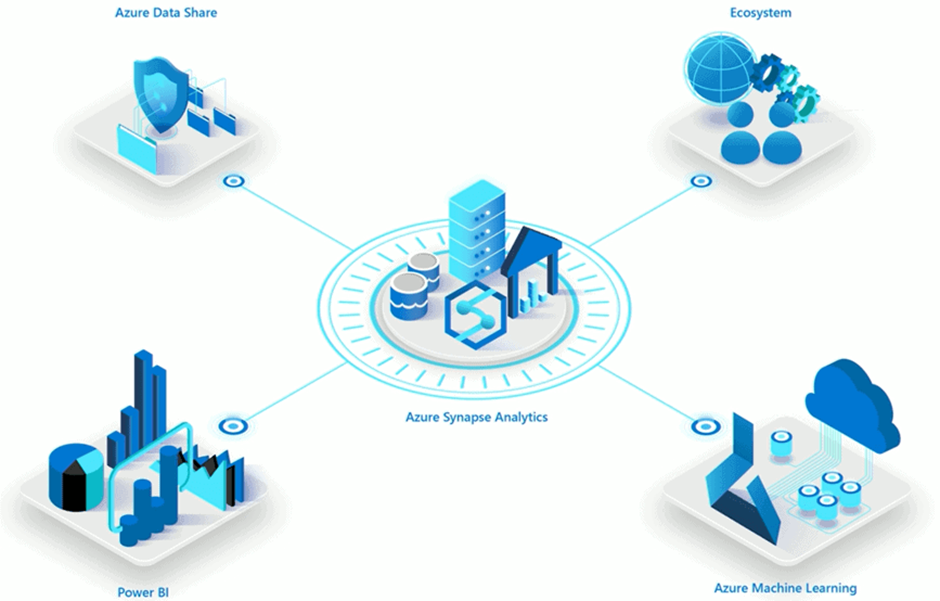
2.    What is Azure Synapse analytics?

As of my last update in September 2021, Azure Synapse Analytics is an integrated analytics service provided by Microsoft as part of the Azure cloud platform. It combines big data and data warehousing capabilities into a single solution, enabling organizations to ingest, prepare, manage, and serve data for business intelligence, machine learning, and real-time analytics purposes. Azure Synapse Analytics was formerly known as Azure SQL Data Warehouse but was rebranded and expanded to offer more comprehensive analytics capabilities.

1. Unified Data Platform: It brings together data integration, data warehousing, big data analytics, and data exploration capabilities into a single unified platform, allowing users to work with diverse data sources seamlessly.

Key features of Azure Synapse Analytics include:

2. Data Integration: Azure Synapse Analytics provides built-in connectors and integration with various data sources, both on-premises and in the cloud, making it easier to ingest and process data from different systems.

3. Data Warehousing: It offers a distributed, scalable, and fully managed data warehousing solution to store and manage large volumes of structured and semi-structured data.

4. Big Data Analytics: The service allows users to perform big data analytics using Apache Spark, enabling data engineers and data scientists to analyze and process large datasets efficiently.

5. Real-time Analytics: Azure Synapse Analytics can be integrated with Azure Stream Analytics, enabling real-time data ingestion and analytics for streaming data scenarios.

6. Machine Learning Integration: It integrates with Azure Machine Learning, facilitating the deployment and operationalization of machine learning models on large datasets.

7. Serverless On-Demand Queries: Users can run serverless SQL queries on data residing in various locations, making it easier to analyze data without requiring a dedicated data warehouse.

8. Power BI Integration: Azure Synapse Analytics seamlessly integrates with Power BI, Microsoft’s business analytics service, enabling users to create interactive reports and dashboards.

9. Security and Governance: The service provides robust security features, including role-based access control, encryption, and data masking, ensuring data privacy and compliance with industry standards.

Overall, Azure Synapse Analytics is designed to provide an end-to-end analytics solution for modern data-driven businesses, allowing them to gain insights from large and diverse datasets efficiently and effectively. However, please note that Microsoft may have introduced new features or updates to Azure Synapse Analytics beyond my last update, so it’s always a good idea to refer to the official Azure documentation for the most current information.

3. Explain the data masking feature of Azure?

Data masking in Azure is a security feature that helps protect sensitive information by obfuscating or hiding sensitive data from unauthorized users or applications. It is an essential part of data security and compliance strategies, ensuring that only authorized individuals can access the actual sensitive data while others are provided with masked or scrambled representations.

Azure provides various tools and services to implement data masking, and one of the primary services used for this purpose is Azure SQL Database. Here’s an overview of how data masking works in Azure:

1. Sensitive Data Identification: The first step in data masking is to identify the sensitive data that needs protection. This includes personally identifiable information (PII), financial data, healthcare data, or any other information that could pose a risk if accessed by unauthorized users.

2. Data Masking Rules: Once sensitive data is identified, data masking rules are defined to specify how the data should be masked. These rules can vary based on the type of data and the level of security required. For example, data might be partially masked, fully masked, or substituted with random characters.

3. Data Masking Operations: When data masking is enabled, the data in the specified columns is automatically masked based on the defined rules. This process happens at the database level, ensuring that applications and users interacting with the database only see the masked data.

4. Access Control: Access control mechanisms, such as role-based access control (RBAC) and permissions, are used to ensure that only authorized users have access to the original (unmasked) data. Access to the masked data is typically provided to users who do not require access to the actual sensitive information.

5. Dynamic Data Masking: In some cases, dynamic data masking is used, which allows administrators to define masking rules dynamically at query runtime based on the user’s privileges. This means that different users may see different masked versions of the data based on their access rights.

Data masking is particularly beneficial in scenarios where developers, testers, or support personnel need access to production data for testing or troubleshooting purposes but should not be exposed to actual sensitive information. By using data masking, organizations can strike a balance between data privacy and the practical need to use realistic datasets for various purposes.

It’s important to note that while data masking provides an additional layer of security, it is not a substitute for robust access controls, encryption, or other security measures. A comprehensive data security strategy should include multiple layers of protection to safeguard sensitive information throughout its lifecycle.

4. Difference between Azure Synapse Analytics and Azure Data Lake Storage?

Feature	Azure Synapse Analytics	Azure Data Lake Storage
Primary Purpose	Unified analytics service that combines big data and data warehousing capabilities.	Scalable and secure data lake storage for storing and managing large volumes of structured and unstructured data.
Data Processing	Provides data warehousing, big data analytics (using Apache Spark), and real-time data processing.	Primarily focused on storing and managing data; data processing is typically performed using separate services or tools.
Data Integration	Offers built-in connectors for integrating data from various sources for analysis.	Primarily focused on data storage, but data can be ingested and processed using other Azure services like Data Factory or Databricks.
Query Language	Supports T-SQL (Transact-SQL) for querying structured data and Apache Spark SQL for big data analytics.	No built-in query language; data is typically accessed and processed through other Azure services or tools.
Data Organization	Organizes data into dedicated SQL data pools and Apache Spark pools for different types of analytics.	Organizes data into hierarchical directories and folders, suitable for storing raw and processed data.
Data Security	Provides robust security measures for data protection, access control, and auditing.	Offers granular access control through Azure Active Directory, and data can be encrypted at rest and in transit.
Schema Management	Requires structured data with a predefined schema for SQL-based analytics.	Supports both structured and unstructured data, allowing schema-on-read for flexible data processing.
Use Cases	Suitable for data warehousing, big data analytics, and real-time analytics scenarios.	Ideal for big data storage, data exploration, data archiving, and serving as a data source for various data processing workloads.
Integration with Other Services	Integrates with other Azure services like Power BI, Azure Machine Learning, and Azure Stream Analytics.	Can be integrated with various Azure services like Data Factory, Databricks, and Azure HDInsight for data processing.

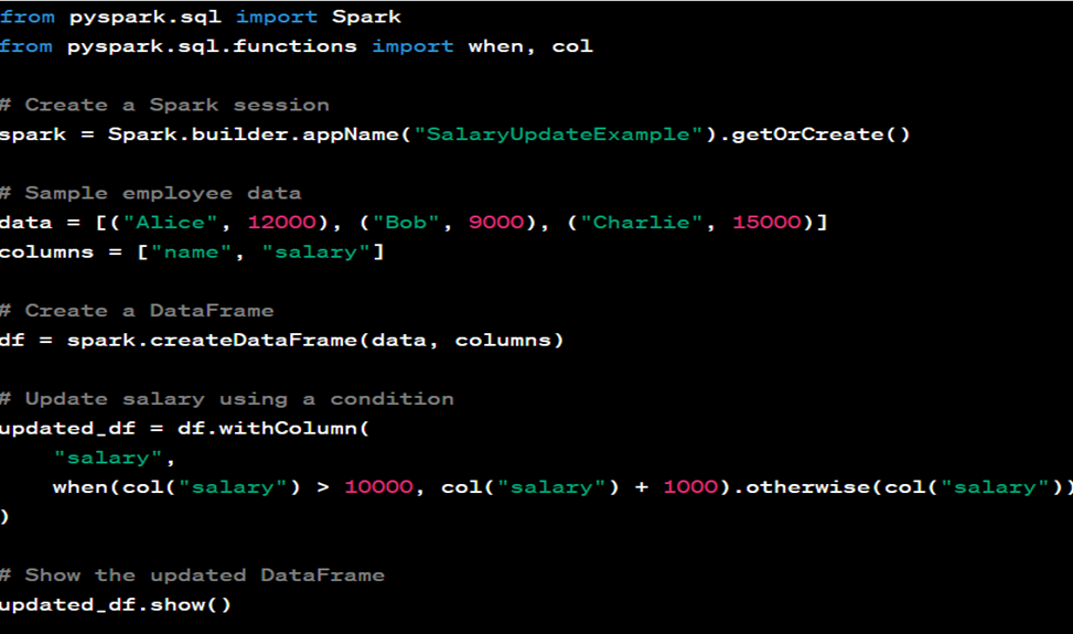
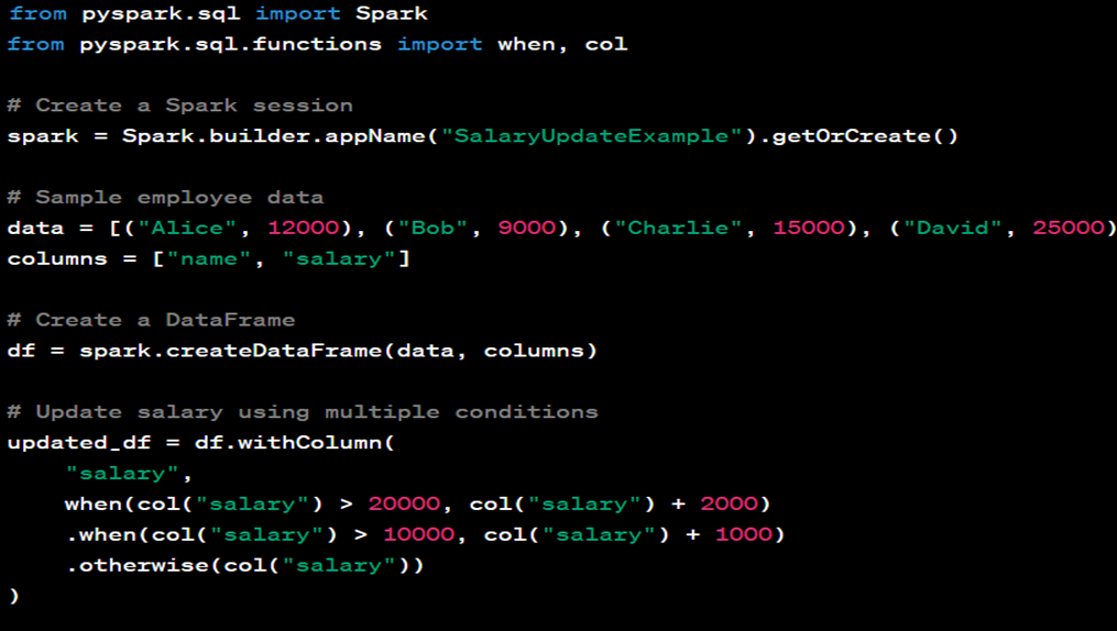
5. Describe various windowing functions of Azure Stream Analytics?

Azure Stream Analytics provides several windowing functions that help you perform calculations on data streams within specific time or event intervals. These functions enable you to perform time-based aggregations, sliding window computations, and more. Here are some of the key windowing functions available in Azure Stream Analytics:

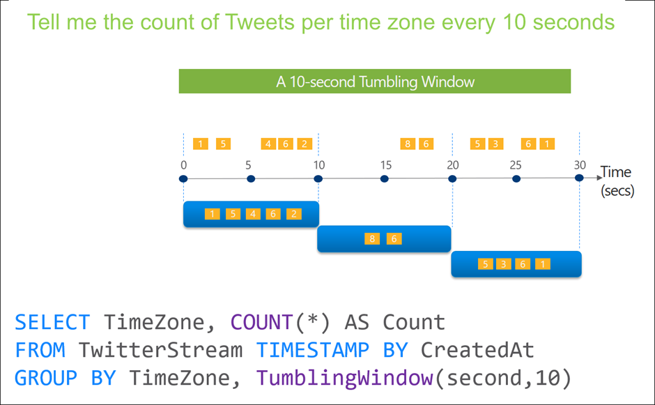
Tumbling Windows:

• Tumbling windows divide the data stream into fixed-size, non-overlapping time intervals.
• Each event belongs to one and only one tumbling window based on its timestamp.
• Useful for performing time-based aggregations over distinct time intervals.

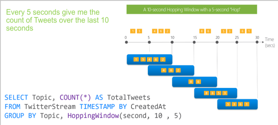
Hopping window

• Hopping windows are similar to tumbling windows but allow overlapping time intervals.
• You can specify the hop size and window size, determining how much overlap exists between adjacent windows.
• Useful for calculating aggregates over sliding time intervals.

Sliding window

• Sliding windows divide the data stream into fixed-size, overlapping time intervals.
• Unlike hopping windows, sliding windows always have an overlap between adjacent windows.
• You can specify the window size and the slide size.
• Useful for analyzing recent data while considering historical context.

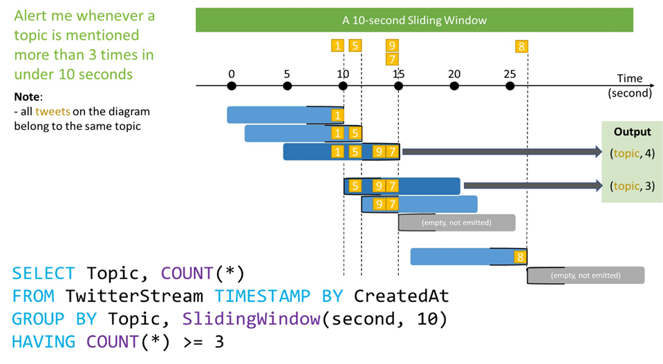
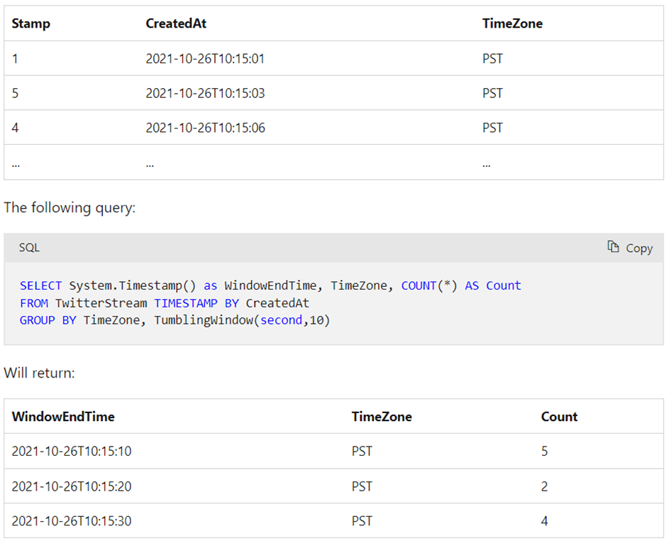
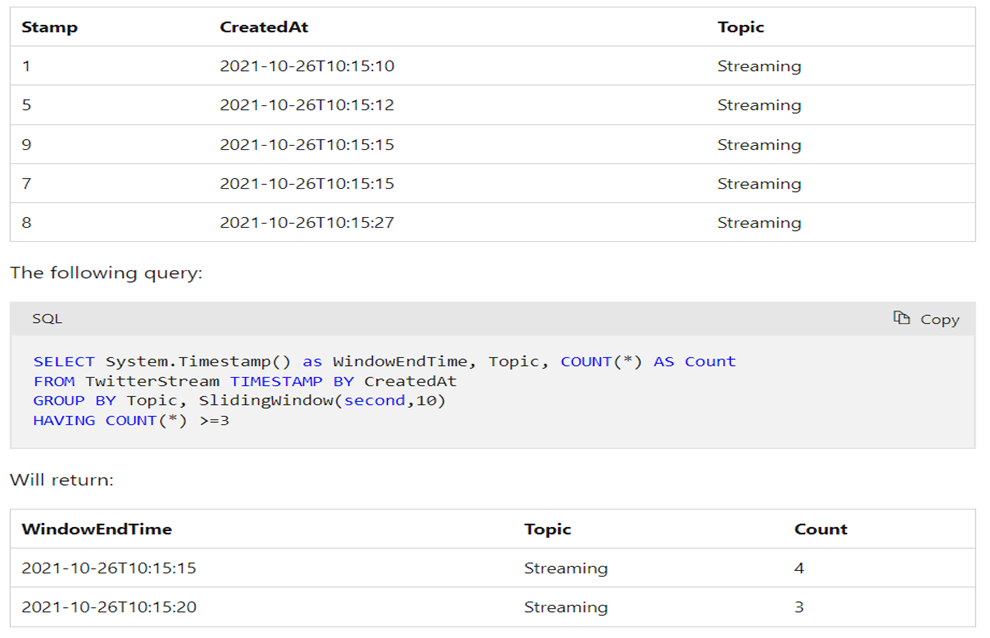
With the following input data (illustrated above):

Session Windows:

• Session windows group events that are close together in time based on a specified gap duration.
• The gap duration is the maximum time interval between events that belong to the same session window.
• Useful for detecting and analyzing bursts or periods of activity in data streams.

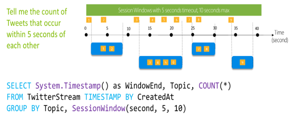
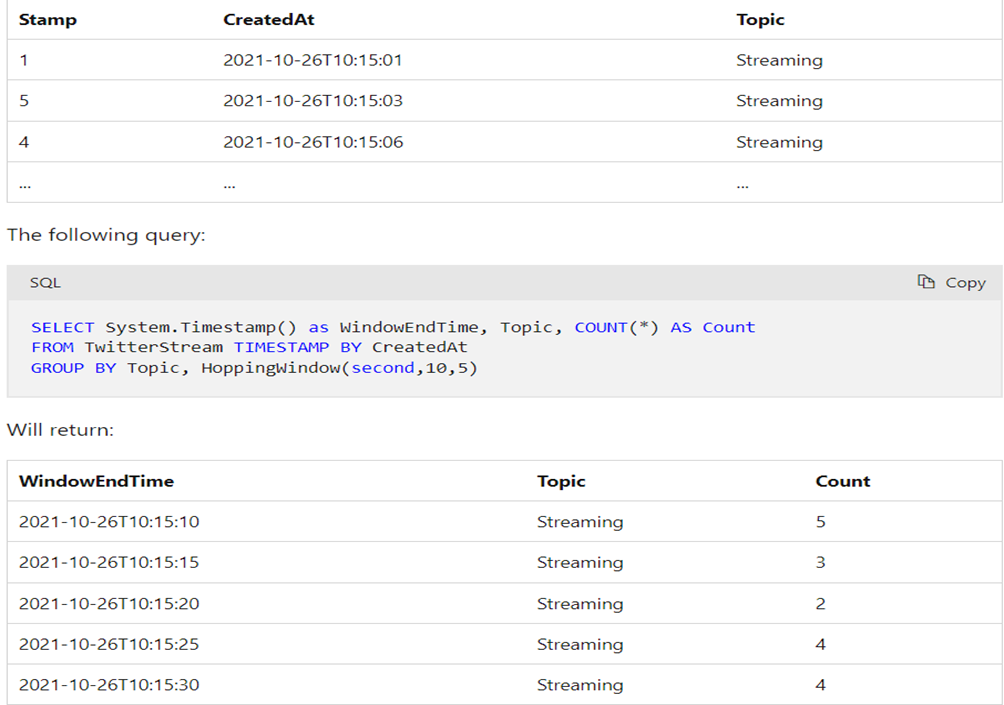
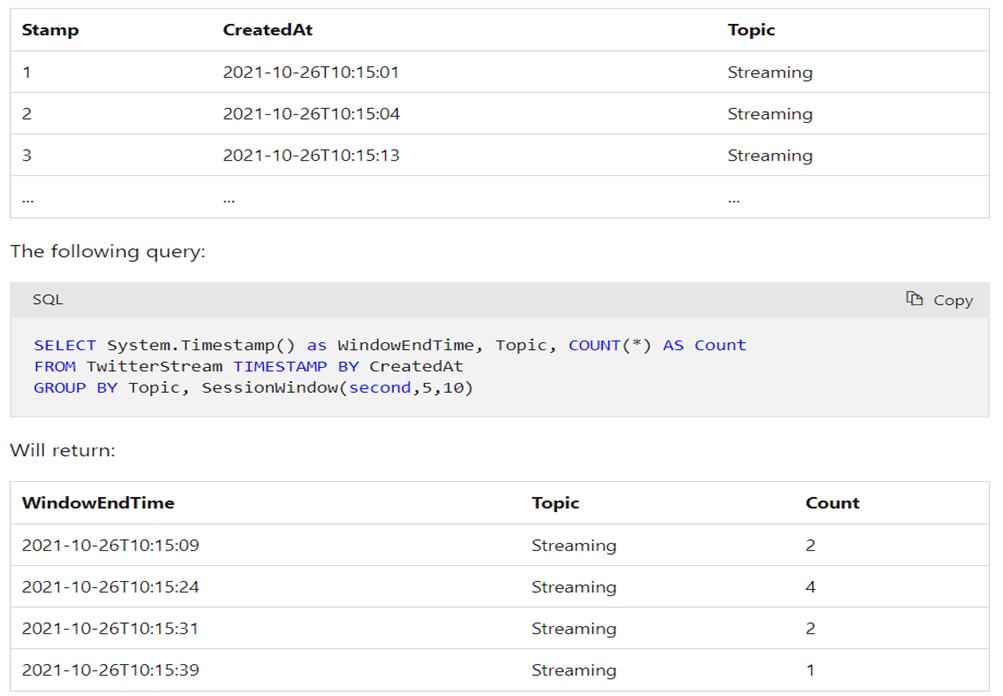
With the following input data (illustrated above):

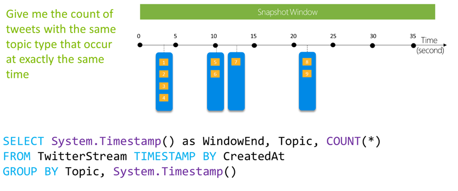
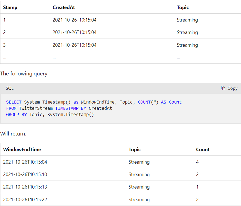
Snapshot window

Snapshot windows group events that have the same timestamp. Unlike other windowing types, which require a specific window function (such as SessionWindow()), you can apply a snapshot window by adding System.Timestamp() to the GROUP BY clause.

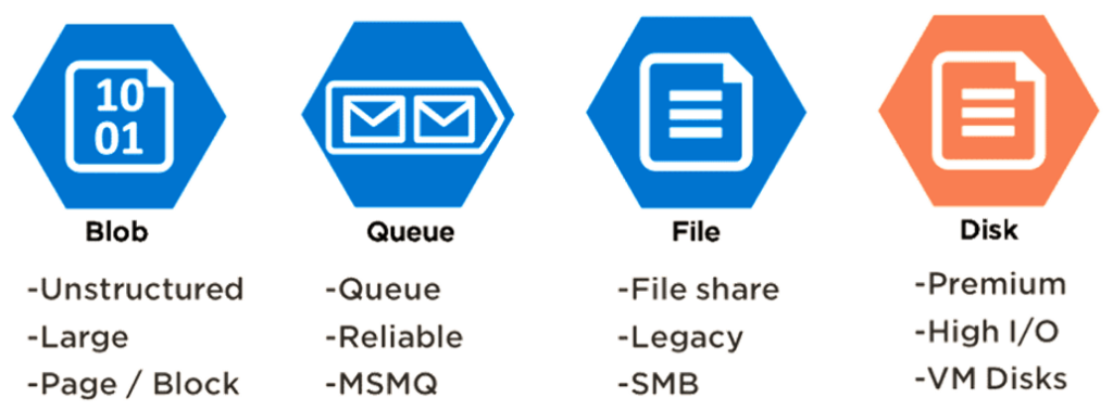
6. What are the different storage types in Azure?

The following are the various advantages of the Java collection framework:

Storage Types	Operations
Files	Azure Files is an organized way of storing data on the cloud. The main advantage of using Azure Files over Azure Blobs is that Azure Files allows for organizing the data in a folder structure. Also, Azure Files is SMB (Server Message Block) protocol compliant, i.e., and can be used as a file share.
Blobs	Blob stands for a large binary object. This storage solution supports all kinds of files, including text files, videos, images, documents, binary data, etc.
Queues	Azure Queue is a cloud-based messaging store for establishing and brokering communication between various applications and components.
Disks	The Azure disk is used as a storage solution for Azure VMs (Virtual Machines)
Tables	Tables are NoSQL storage structures for storing structured data that does not meet the standard RDBMS (relational database schema).

7. What are the different security options available in the Azure SQL database?

Azure SQL Database provides a range of security options to ensure the confidentiality, integrity, and availability of your data. These options are designed to protect your database from unauthorized access, data breaches, and other security threats. Here are some of the key security features available in Azure SQL Database:

1. Firewall Rules:

• Azure SQL Database allows you to configure firewall rules to control which IP addresses or IP address ranges can access your database.
• By default, all access from outside Azure’s datacenters is blocked until you define the necessary firewall rules.

2. Authentication:

• Azure SQL Database supports two types of authentications: SQL Authentication and Azure Active Directory Authentication.
• SQL Authentication uses usernames and passwords to authenticate users, while Azure Active Directory Authentication enables users to sign in with their Azure AD credentials.

3. Transparent Data Encryption (TDE):

• TDE automatically encrypts data at rest, providing an additional layer of security for your database.
• The data and log files are encrypted using a database encryption key, which is further protected by a service-managed certificate.

4. Always Encrypted:

• Always Encrypted is a feature that allows you to encrypt sensitive data in the database while keeping the encryption keys within your application.
• This ensures that even database administrators cannot access the plaintext data.

5. Auditing and Threat Detection:

• Azure SQL Database offers built-in auditing that allows you to track database events and store audit logs in Azure Storage.
• Threat Detection provides continuous monitoring and anomaly detection to identify potential security threats and suspicious activities.

6. Row-Level Security (RLS):

• RLS enables you to control access to rows in a database table based on the characteristics of the user executing a query.
• This feature is useful for implementing fine-grained access controls on a per-row basis.

7. Virtual Network Service Endpoints:

• With Virtual Network Service Endpoints, you can extend your virtual network’s private IP address space and route traffic securely to Azure SQL Database over the Azure backbone network.
• This helps to ensure that your database can only be accessed from specific virtual networks, improving network security.

8. Data Masking:

• Data Masking enables you to obfuscate sensitive data in query results, making it possible to share the data with non-privileged users without revealing the actual values.

9. Threat Protection:

• Azure SQL Database’s Threat Protection feature helps identify and mitigate potential database vulnerabilities and security issues.

10. Advanced Data Security (ADS):

• Advanced Data Security is a unified package that includes features like Vulnerability Assessment, Data Discovery & Classification, and SQL Injection Protection to enhance the overall security of your database.

By leveraging these security options, you can ensure that your Azure SQL Database remains protected against various security threats and maintain the confidentiality and integrity of your data. It is essential to configure and monitor these security features based on your specific requirements and compliance standards.

8. How data security is implemented in Azure Data Lake Storage(ADLS) Gen2?

Azure Data Lake Storage Gen2 (ADLS Gen2) provides robust data security features to protect data at rest and in transit. It builds on the security features of Azure Blob Storage and adds hierarchical namespace support, enabling it to function as both an object store and a file system. Here’s how data security is implemented in Azure Data Lake Storage Gen2:

1. Role-Based Access Control (RBAC):

• ADLS Gen2 leverages Azure RBAC to control access to resources at the Azure subscription and resource group levels.
• You can assign roles such as Storage Account Contributor, Storage Account Owner, or Custom roles with specific permissions to users, groups, or applications.

2. POSIX Access Control Lists (ACLs):

• ADLS Gen2 supports POSIX-like ACLs, allowing you to grant fine-grained access control to individual files and directories within the data lake.
• This enables you to define access permissions for specific users or groups, controlling read, write, and execute operations.

3. Shared Access Signatures (SAS):

• SAS tokens provide limited and time-bound access to specific resources in ADLS Gen2.
• You can generate SAS tokens with custom permissions and time constraints, which are useful for granting temporary access to external entities without exposing storage account keys.

4. Data Encryption:

• Data at rest is automatically encrypted using Microsoft-managed keys (SSE, Server-Side Encryption).
• Optionally, you can bring your encryption keys using customer-managed keys (CMEK) for an added layer of control.

5. Azure Private Link:

• ADLS Gen2 can be integrated with Azure Private Link, which allows you to access the service over a private, dedicated network connection (Azure Virtual Network).
• This helps to prevent data exposure to the public internet and enhances network security.

6. Firewall and Virtual Network Service Endpoints:

• ADLS Gen2 allows you to configure firewall rules to control which IP addresses or IP address ranges can access the data lake.
• Virtual Network Service Endpoints enable secure access to the data lake from within an Azure Virtual Network.

7. Data Classification and Sensitivity Labels:

• ADLS Gen2 supports Azure Data Classification and Sensitivity Labels, allowing you to classify and label data based on its sensitivity level.
• These labels can be used to enforce policies, auditing, and access control based on data classification.

8. Auditing and Monitoring:

• ADLS Gen2 offers auditing capabilities that allow you to track access to the data lake and log events for compliance and security monitoring.
• You can integrate ADLS Gen2 with Azure Monitor to get insights into the health and performance of the service.

By combining these security features, Azure Data Lake Storage Gen2 ensures that your data is protected from unauthorized access, tampering, and data breaches. It is crucial to configure these security options based on your specific data security requirements and compliance standards to safeguard your data effectively.

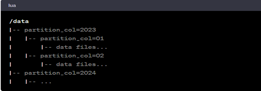
9. What are the various data flow partition schemes available in Azure?

Partition Scheme	Explanation	Usage
Round Robin	It is the most straightforward partition scheme which spreads data evenly across partitions.	No good key candidates were available in the data.
Hash	Hash of columns creates uniform partitions such that rows with similar values fall in the same partition.	It is used to check for partition skew.
Dynamic Range	Spark dynamics range based on the provided columns or expression.	Select the column that will be used for partitioning.
Fixed Range	A fixed range of values based on the user-created expression for disturbing data across partitions.	A good understanding of data is required to avoid partition skew.
Key	Partition for each unique value in the selected column.	Good understanding of data cardinality is required.

10. Why is the Azure data factory needed?

Azure Data Factory is a cloud-based data integration service provided by Microsoft Azure. It is designed to address the challenges of data movement and data orchestration in modern data-centric environments. The primary reasons why Azure Data Factory is needed are as follows:

1. Data Integration and Orchestration: In today’s data landscape, organizations often deal with data spread across various sources and formats, both on-premises and in the cloud. Azure Data Factory enables seamless integration and orchestration of data from diverse sources, making it easier to collect, transform, and move data between systems.

2. ETL (Extract, Transform, Load) Workflows: ETL processes are fundamental in data warehousing and analytics. Azure Data Factory allows you to create complex data workflows, where you can extract data from different sources, apply transformations, and load it into the target destination efficiently.

3. Serverless and Scalable: Azure Data Factory is a serverless service, meaning you don’t need to manage the underlying infrastructure. It automatically scales up or down based on demand, ensuring that you can process data of any volume without worrying about infrastructure limitations.

4. Integration with Azure Services: As part of the Azure ecosystem, Data Factory seamlessly integrates with other Azure services like Azure Blob Storage, Azure SQL Database, Azure Data Lake, Azure Databricks, etc. This integration enhances data processing capabilities and enables users to take advantage of Azure’s broader suite of analytics and storage solutions.

5. Data Transformation and Data Flow: Azure Data Factory provides data wrangling capabilities through data flows, allowing users to build data transformation logic visually. This simplifies the process of data cleansing, enrichment, and preparation for analytics or reporting.

6. Monitoring and Management: Azure Data Factory comes with built-in monitoring and management tools that allow you to track the performance of your data pipelines, troubleshoot issues, and set up alerts for critical events.

7. Hybrid Data Movement: For organizations with a hybrid cloud strategy or data stored on-premises, Azure Data Factory offers connectivity to on-premises data sources using a secure data gateway. This enables smooth integration of cloud and on-premises data.

8. Time Efficiency: Data Factory enables you to automate data pipelines and schedule data movements and transformations, reducing manual intervention and saving time in the data integration process.

Overall, Azure Data Factory plays a crucial role in simplifying data integration, enabling organizations to gain insights from their data, and facilitating the development of robust data-driven solutions in the Azure cloud environment.

11. What is Azure Data Factory?

Azure Data Factory is a cloud-based integration service offered by Microsoft that lets you create data-driven workflows for orchestrating and automating data movement and data transformation overcloud. Data Factory services also offer to create and running data pipelines that move and transform data and then run the pipeline on a specified schedule.

12. What is Integration Runtime?

Integration runtime is nothing but a compute structure used by Azure Data Factory to give integration capabilities across different network environments.

Types of Integration Runtimes:

• Azure Integration Runtime – It can copy data between cloud data stores and dispatch the activity to a variety of computing services such as SQL Server, Azure HDInsight
• Self Hosted Integration Runtime – It’s software with basically the same code as Azure Integration runtime, but it’s installed on on- premises systems or virtual machines over virtual networks.
• Azure SSIS Integration Runtime – It helps to execute SSIS packages in a managed environment. So when we lift and shift the SSIS packages to the data factory, we use Azure SSIS Integration Runtime.

13. What are the different components used in Azure Data Factory?

Azure Data Factory consists of several numbers of components. Some components are as follows:

• Pipeline: The pipeline is the logical container of the activities.
• Activity: It specifies the execution step in the Data Factory pipeline, which is substantially used for data ingestion and metamorphosis.
• Dataset: A dataset specifies the pointer to the data used in the pipeline conditioning.
• Mapping Data Flow: It specifies the data transformation UI logic.
• Linked Service: It specifies the descriptive connection string for the data sources used in the channel conditioning.  Let‘s say we’ve an SQL server, so we need a connecting string connected to an external device, and we will mention the source and the destination for it.
• Trigger: It specifies the time when the pipeline will be executed.
• Control flow: It’s used to control the execution flow of the pipeline activities

14. What is the key difference between the Dataset and Linked Service in Azure Data Factory?

Dataset specifies a source to the data store described by the linked service. When we put data to the dataset from a SQL Server instance, the dataset indicates the table’s name that contains the target data or the query that returns data from dissimilar tables.

Linked service specifies a definition of the connection string used to connect to the data stores. For illustration, when we put data in a linked service from a SQL Server instance, the linked service contains the name for the SQL Server instance and the credentials used to connect to that case.

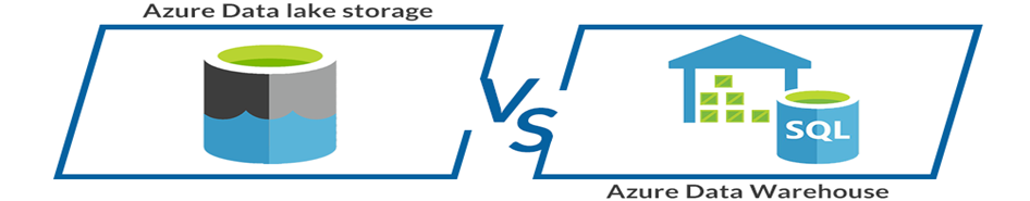
15. What is the difference between Azure Data Lake and Azure Data Warehouse?

Azure Data Lake	Data Warehouse
Data Lake is a capable way of storing any type, size, and shape of data.	Data Warehouse acts as a repository for already filtered data from a specific resource.
It is mainly used by Data Scientists.	It is more frequently used by Business Professionals.
It is highly accessible with quicker updates.	It becomes a pretty rigid and costly task to make changes in Data Warehouse.
It defines the schema after when the data is stored successfully.	Datawarehouse defines the schema before storing the data.
It uses ELT (Extract, Load and Transform) process.	It uses ETL (Extract, Transform and Load) process.
It is an ideal platform for doing in-depth analysis.	It is the best platform for operational users.

16. Difference between Data Lake Storage and Blob Storage.

Data Lake Storage	Blob Storage
It is an optimized storage solution for big data analytics workloads.	Blob Storage is general-purpose storage for a wide variety of scenarios. It can also do Big Data Analytics.
It follows a hierarchical file system.	It follows an object store with a flat namespace.
In Data Lake Storage, data is stored as files inside folders.	Blob storage lets you create a storage account. Storage account has containers that store the data.
It can be used to store Batch, interactive, stream analytics,  and machine learning data.	We can use it to store text files, binary data, media storage for streaming and general purpose data.

16. What are the steps to create an ETL process in Azure Data Factory?

The ETL (Extract, Transform, Load) process follows four main steps:

i) Connect and Collect: Connect to the data source/s and move data to local and crowdsource data storage.

ii) Data transformation using computing services such as HDInsight, Hadoop, Spark, etc.

iii) Publish: To load data into Azure data lake storage, Azure SQL data warehouse, Azure SQL databases, Azure Cosmos DB, etc.

iv)Monitor: Azure Data Factory has built-in support for pipeline monitoring via Azure Monitor, API, PowerShell, Azure Monitor logs, and health panels on the Azure portal.

17. What are the key differences between the Mapping data flow and Wrangling data flow transformation activities in Azure Data Factory?

In Azure Data Factory, the main dissimilarity between the Mapping data flow and the Wrangling data flow transformation activities is as follows

The Mapping data flow activity is a visually allowed data transformation activity that facilitates users to plan graphical data transformation logic. It does not need the users to be expert developers. It’s executed as an activity within the ADF pipeline on an ADF completely managed scaled-out Spark cluster.

On the other hand, the Wrangling data flow activity is a code–free data preparation activity. It’s integrated with Power Query Online to make the Power Query M functions available for data wrangling using spark execution.

18. Can we pass parameters to a pipeline run?

Yes definitely, we can very easily pass parameters to a pipeline run. Pipeline runs are the first-class, top-level concepts in Azure Data Factory. We can define parameters at the pipeline level, and then we can pass the arguments to run a pipeline.

You can also define default values for the parameters in the pipeline.

19. Can an activity in a pipeline consume arguments that are passed to a pipeline run?

Each activity within the pipeline can consume the parameter value that’s passed to the pipeline and run with the @parameter construct.

Parameters are a first-class, top-level concept in Data Factory. We can define parameters at the pipeline level and pass arguments as you execute the pipeline run on demand or using a trigger. 

20. Can an activity output property be consumed in another activity?

An activity output can be consumed in a subsequent activity with the @activity construct.

21. How do I gracefully handle null values in an activity output?

You can use the @coalesce construct in the expressions to handle the null values gracefully.

23. What has changed from private preview to limited public preview in regard to data flows?

There are a couple of things which have been changed mentioned below:

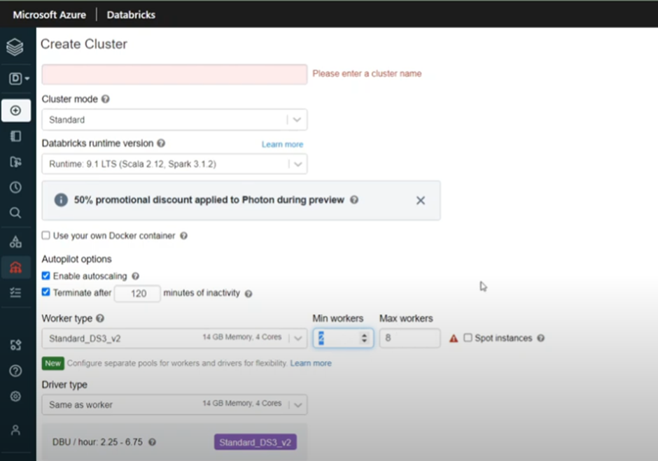
• You are no longer required to bring your own Azure Databricks Clusters.
• Data Factory will manage cluster creation and tear down process.
• We can still use Data Lake Storage Gen 2 and Blob Storage to store those files. You can use the appropriate linked services. You can also use the appropriate linked services for those of the storage engines.
• Blob data sets and Azure Data Lake storage gen 2 are separated into delimited text and Apache Parquet datasets.

24. What is Azure SSIS Integration Runtime?

Azure SSIS Integration is a fully managed cluster of virtual machines that are hosted in Azure and dedicated to run SSIS packages in the data factory. We can easily scale up the SSIS nodes by configuring the node size or scaled out by configuring the number of nodes on the Virtual Machine’s cluster.

We must create an SSIS integration runtime and an SSISDB catalog hosted in the Azure SQL server database or Azure SQL-managed instance before executing an SSIS package

25. An Azure Data Factory Pipeline can be executed using three methods. Mention these methods.

Methods to execute Azure Data Factory Pipeline:

• Debug Mode
• Manual execution using trigger now
• Adding schedule, tumbling window/event trigger

26. Can we monitor and manage Azure Data Factory Pipelines?

Yes, we can monitor and manage ADF Pipelines using the following steps:

• Click on the monitor and manage on the data factory tab.
• Click on the resource manager.
• Here, you will find- pipelines, datasets, and linked services in a tree format.

27. What are the steps involved in the ETL process?

ETL (Extract, Transform, Load) process follows four main steps:

• Connect and Collect – helps in moving the data on-premises and cloud source data stores
• Transform – lets users collect the data by using compute services such as HDInsight Hadoop, Spark etc.
• Publish – Helps in loading the data into Azure data warehouse, Azure SQL database, and Azure Cosmos DB etc
• Monitor – It helps support the pipeline monitoring via Azure Monitor, API and PowerShell, Log Analytics, and health panels on the Azure Portal.

28. What are the different ways to execute pipelines in Azure Data Factory?

There are three ways in which we can execute a pipeline in Data Factory:

• Debug mode can be helpful when trying out pipeline code and acts as a tool to test and troubleshoot our code.
• Manual Execution is what we do by clicking on the ‘Trigger now’ option in a pipeline. This is useful if you want to run your pipelines on an ad-hoc basis.
• We can schedule our pipelines at predefined times and intervals via a Trigger. As we will see later in this article, there are three types of triggers available in Data Factory. 

29. What is the purpose of Linked services in Azure Data Factory?

Linked services are used majorly for two purposes in Data Factory:

1. For a Data Store representation, i.e., any storage system like Azure Blob storage account, a file share, or an Oracle DB/ SQL Server instance.
2.  For Compute representation, i.e., the underlying VM will execute the activity defined in the pipeline. 

30. Can you Elaborate more on Data Factory Integration Runtime?

The Integration Runtime, or IR, is the compute infrastructure for Azure Data Factory pipelines. It is the bridge between activities and linked services. The linked Service or Activity references it and provides the computing environment where the activity is run directly or dispatched. This allows the activity to be performed in the closest region to the target data stores or computing Services.

The following diagram shows the location settings for Data Factory and its integration runtimes:

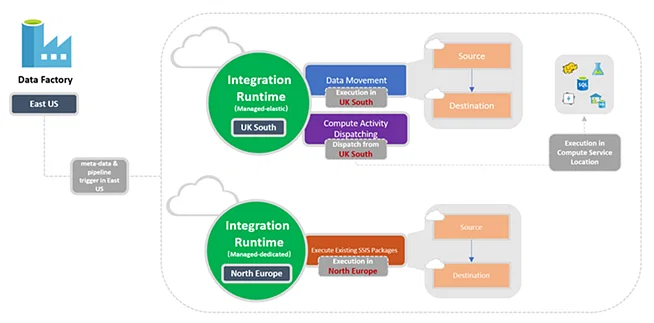
Azure Data Factory supports three types of integration runtime, and one should choose based on their data integration capabilities and network environment requirements.

1. Azure Integration Runtime: To copy data between cloud data stores and send activity to various computing services such as SQL Server, Azure HDInsight, etc.
2. Self-Hosted Integration Runtime: Used for running copy activity between cloud data stores and data stores in private networks. Self-hosted integration runtime is software with the same code as the Azure Integration Runtime but installed on your local system or machine over a virtual network. 
3. Azure SSIS Integration Runtime: You can run SSIS packages in a managed environment. So, when we lift and shift SSIS packages to the data factory, we use Azure SSIS Integration Runtime. 

31. What are ARM Templates in Azure Data Factory? What are they used for?

An ARM template is a JSON (JavaScript Object Notation) file that defines the infrastructure and configuration for the data factory pipeline, including pipeline activities, linked services, datasets, etc. The template will contain essentially the same code as our pipeline.

ARM templates are helpful when we want to migrate our pipeline code to higher environments, say Production or Staging from Development, after we are convinced that the code is working correctly.

32. What are the two types of compute environments supported by Data Factory to execute the transform activities?

Below are the types of computing environments that Data Factory supports for executing transformation activities: –

i) On-Demand Computing Environment: This is a fully managed environment provided by ADF. This type of calculation creates a cluster to perform the transformation activity and automatically deletes it when the activity is complete.

ii) Bring Your Environment: In this environment, you can use ADF to manage your computing environment if you already have the infrastructure for on-premises services. 

33. If you want to use the output by executing a query, which activity shall you use? 

Look-up activity can return the result of executing a query or stored procedure.

The output can be a singleton value or an array of attributes, which can be consumed in subsequent copy data activity, or any transformation or control flow activity like ForEach activity.

34. What are some useful constructs available in Data Factory?

• parameter: Each activity within the pipeline can consume the parameter value passed to the pipeline and run with the @parameter construct.
• coalesce: We can use the @coalesce construct in the expressions to handle null values gracefully.
• activity: An activity output can be consumed in a subsequent activity with the            @activity construct. 

35. Can we push code and have CI/CD (Continuous Integration and Continuous Delivery) in ADF?

Data Factory fully supports CI/CD of your data pipelines using Azure DevOps and GitHub. This allows you to develop and deliver your ETL processes incrementally before publishing the finished product. After the raw data has been refined into a business-ready consumable form, load the data into Azure Data Warehouse or Azure SQL Azure Data Lake, Azure Cosmos DB, or whichever analytics engine your business uses can point to from their business intelligence tools.

36. What do you mean by variables in the Azure Data Factory?

Variables in the Azure Data Factory pipeline provide the functionality to hold the values. They are used for a similar reason as we use variables in any programming language and are available inside the pipeline.

Set variables and append variables are two activities used for setting or manipulating the values of the variables. There are two types of variables in a data factory: –

i) System variables:  These are fixed variables from the Azure pipeline. For example, pipeline name, pipeline id, trigger name, etc. You need these to get the system information required in your use case.

ii) User variable: A user variable is declared manually in your code based on your pipeline logic.

37. What are the different activities you have used in Azure Data Factory?

Here you can share some of the significant activities if you have used them in your career, whether your work or college project. Here are a few of the most used activities :

1. Copy Data Activity to copy the data between datasets.
2. ForEach Activity for looping.
3. Get Metadata Activity that can provide metadata about any data source.
4. Set Variable Activity to define and initiate variables within pipelines.
5. Lookup Activity to do a lookup to get some values from a table/file.
6. Wait Activity to wait for a specified amount of time before/in between the pipeline run.
7. Validation Activity will validate the presence of files within the dataset.
8. Web Activity to call a custom REST endpoint from an ADF pipeline.

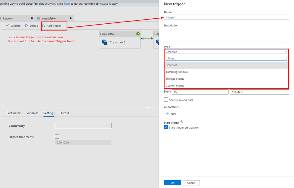
38. How can I schedule a pipeline?

You can use the time window or scheduler trigger to schedule a pipeline. The trigger uses a wall-clock calendar schedule, which can schedule pipelines periodically or in calendar-based recurrent patterns (for example, on Mondays at 6:00 PM and Thursdays at 9:00 PM).

 Currently, the service supports three types of triggers:

• Tumbling window trigger: A trigger that operates on a periodic interval while retaining a state.
• Schedule Trigger: A trigger that invokes a pipeline on a wall-clock schedule.
• Event-Based Trigger: A trigger that responds to an event. e.g., a file getting placed inside a blob.
  Pipelines and triggers have a many-to-many relationship (except for the tumbling window trigger). Multiple triggers can kick off a single pipeline, or a single trigger can kick off numerous pipelines.

39. How can you access data using the other 90 dataset types in Data Factory?

The mapping data flow feature allows Azure SQL Database, Azure Synapse Analytics, delimited text files from Azure storage account or Azure Data Lake Storage Gen2, and Parquet files from blob storage or Data Lake Storage Gen2 natively for source and sink data source. Use the Copy activity to stage data from any other connectors and then execute a Data Flow activity to transform data after it’s been staged.

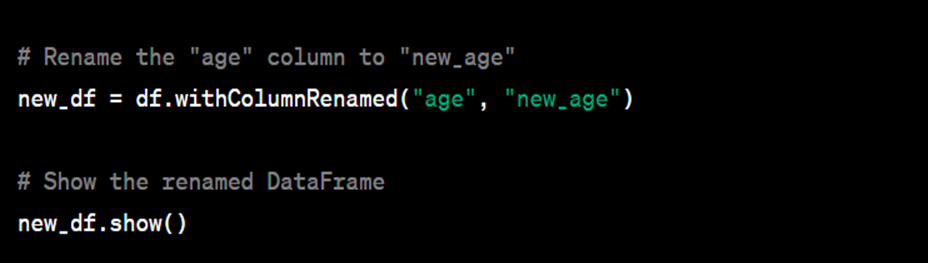
40. Can a value be calculated for a new column from the existing column from mapping in ADF?

We can derive transformations in the mapping data flow to generate a new column based on our desired logic. We can create a new derived column or update an existing one when developing a derived one. Enter the name of the column you’re making in the Column textbox.

You can use the column dropdown to override an existing column in your schema. Click the Enter expression textbox to start creating the derived column’s expression. You can input or use the expression builder to build your logic.

41. How is the lookup activity useful in the Azure Data Factory?

In the ADF pipeline, the Lookup activity is commonly used for configuration lookup purposes, and the source dataset is available. Moreover, it retrieves the data from the source dataset and then sends it as the activity output. Generally, the output of the lookup activity is further used in the pipeline for making decisions or presenting any configuration as a result.

Simply put, lookup activity is used for data fetching in the ADF pipeline. The way you would use it entirely relies on your pipeline logic. Obtaining only the first row is possible, or you can retrieve the complete rows depending on your dataset or query.

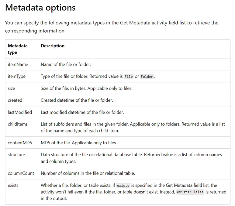
42. Elaborate more on the Get Metadata activity in Azure Data Factory.

The Get Metadata activity is used to retrieve the metadata of any data in the Azure Data Factory or a Synapse pipeline. We can use the output from the Get Metadata activity in conditional expressions to perform validation or consume the metadata in subsequent activities.

It takes a dataset as input and returns metadata information as output. Currently, the following connectors and the corresponding retrievable metadata are supported. The maximum size of returned metadata is 4 MB. 

Please refer to the snapshot below for supported metadata which can be retrieved using the Get Metadata activity.

43. What does it mean by the breakpoint in the ADF pipeline?

To understand better, for example, you are using three activities in the pipeline, and now you want to debug up to the second activity only. You can do this by placing the breakpoint at the second activity. To add a breakpoint, click the circle present at the top of the activity.

44. Can you share any difficulties you faced while getting data from on-premises to Azure cloud using Data Factory?

One of the significant challenges we face while migrating from on-prem to the cloud is throughput and speed. When we try to copy the data using Copy activity from on-prem, the process rate could be faster, and hence we need to get the desired throughput. 

There are some configuration options for a copy activity, which can help in tuning this process and can give desired results.

i) We should use the compression option to get the data in a compressed mode while loading from on-prem servers, which is then de-compressed while writing on the cloud storage.

ii) Staging area should be the first destination of our data after we have enabled the compression. The copy activity can decompress before writing it to the final cloud storage buckets.

iii) Degree of Copy Parallelism is another option to help improve the migration process. This is identical to having multiple threads processing data and can speed up the data copy process.

There is no right fit-for-all here, so we must try different numbers like 8, 16, or 32 to see which performs well.

iv) Data Integration Unit is loosely the number of CPUs used, and increasing it may improve the performance of the copy process. 

45. How to copy multiple sheet data from an Excel file?

When using an Excel connector within a data factory, we must provide a sheet name from which we must load data. This approach is nuanced when we have to deal with a single or a handful of sheets of data, but when we have lots of sheets (say 10+), this may become a tedious task as we have to change the hard-coded sheet name every time!

However, we can use a data factory binary data format connector for this and point it to the Excel file and need not provide the sheet name/s. We’ll be able to use copy activity to copy the data from all the sheets present in the file.

46. Is it possible to have nested looping in Azure Data Factory?

There is no direct support for nested looping in the data factory for any looping activity (for each / until). However, we can use one for each/until loop activity which will contain an execute pipeline activity that can have a loop activity. This way, when we call the looping activity, it will indirectly call another loop activity, and we’ll be able to achieve nested looping.

47. How to copy multiple tables from one datastore to another datastore?

An efficient approach to complete this task would be:

• Maintain a lookup table/ file containing the list of tables and their source, which needs to be copied.
• Then, we can use the lookup activity and each loop activity to scan through the list.
• Inside the for each loop activity, we can use a copy activity or a mapping dataflow to copy multiple tables to the destination datastore.

48. What are some performance-tuning techniques for Mapping Data Flow activity?

We could consider the below set of parameters for tuning the performance of a Mapping Data Flow activity we have in a pipeline.

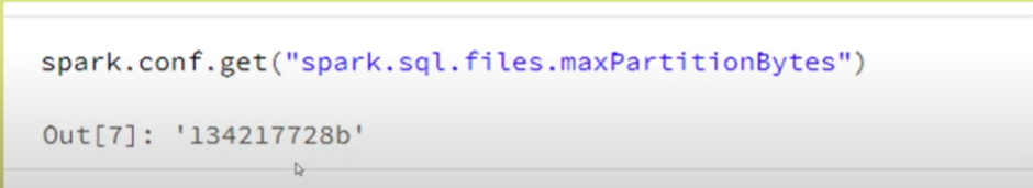
i) We should leverage partitioning in the source, sink, or transformation whenever possible. Microsoft, however, recommends using the default partition (size 128 MB) selected by the Data Factory as it intelligently chooses one based on our pipeline configuration.

Still, one should try out different partitions and see if they can have improved performance.

ii) We should not use a data flow activity for each loop activity. Instead, we have multiple files similar in structure and processing needs. In that case, we should use a wildcard path inside the data flow activity, enabling the processing of all the files within a folder.

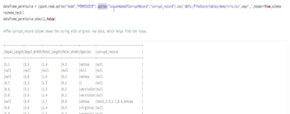
iii) The recommended file format to use is ‘. parquet’. The reason being the pipeline will execute by spinning up spark clusters, and Parquet is the native file format for Apache spark thus, it will generally give good performance.

iv) Multiple logging modes are available: Basic, Verbose, and None.

We should only use verbose mode if essential, as it will log all the details about each operation the activity performs. e.g., It will log all the details of the operations performed for all our partitions. This one is useful when troubleshooting issues with the data flow.

The basic mode will give out all the necessary basic details in the log, so try to use this one whenever possible.

v)  Try to break down a complex data flow activity into multiple data flow activities. Let’s say we have several transformations between source and sink, and by adding more, we think the design has become complex. In this case, try to have it in multiple such activities, which will give two advantages:

• All activities will run on separate spark clusters, decreasing the run time for the whole task.
• The whole pipeline will be easy to understand and maintain in the future. 

49. What are some of the limitations of ADF?

Azure Data Factory provides great functionalities for data movement and transformations. However, there are some limitations as well.

i) We can’t have nested looping activities in the data factory, and we must use some workaround if we have that sort of structure in our pipeline. All the looping activities come under this: If, Foreach, switch, and until activities.

ii) The lookup activity can retrieve only 5000 rows at a time and not more than that. Again, we need to use some other loop activity along with SQL with the limit to achieve this sort of structure in the pipeline.

iii) We can have 40 activities in a single pipeline, including inner activity, containers, etc. To overcome this, we should modularize the pipelines regarding the number of datasets, activities, etc.

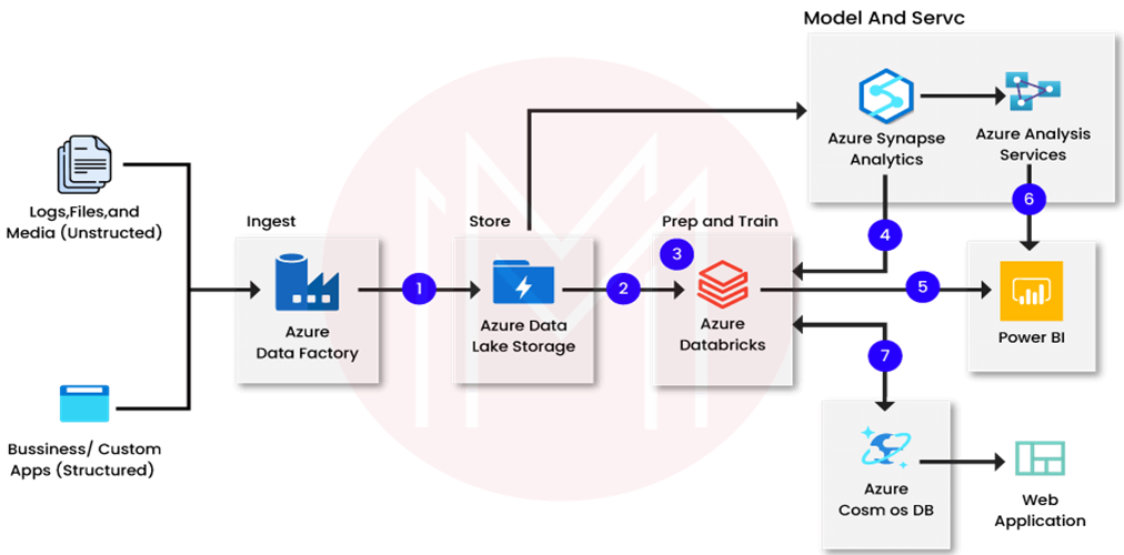
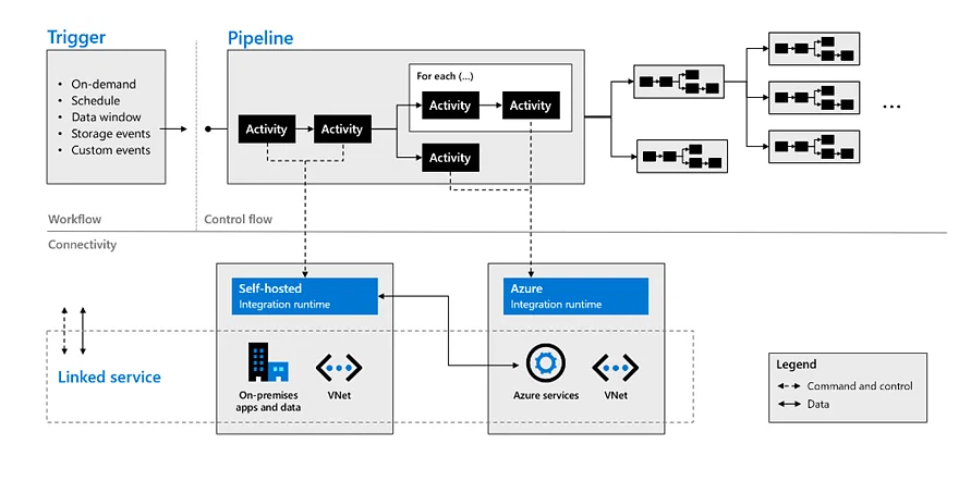
50. How are all the components of Azure Data Factory combined to complete an ADF task?

The below diagram depicts how all these components can be clubbed together to fulfill Azure Data Factory ADF tasks.

51. How do you send email notifications on pipeline failure?

There are multiple ways to do this:

1. Using Logic Apps with Web/Webhook activity.
   Configure a logic app that, upon getting an HTTP request, can send an email to the required set of people for failure. In the pipeline, configure the failure option to hit the URL generated by the logic app.
2. Using Alerts and Metrics from pipeline options.
   We can set up this from the pipeline itself, where we get numerous options for email on any activity failure within the pipeline.

52. Imagine you need to process streaming data in real time and store the results in an Azure Cosmos DB database. How would you design a pipeline in Azure Data Factory to efficiently handle the continuous data stream and ensure it is correctly stored and indexed in the destination database? 

Here are the steps to design a pipeline in Azure Data Factory to efficiently handle streaming data and store it in an Azure Cosmos DB database. 

1. Set up an Azure Event Hub or Azure IoT Hub as the data source to receive the streaming data. 
2. Use Azure Stream Analytics to process and transform the data in real time using Stream Analytics queries.
3. Write the transformed data to a Cosmos DB collection as an output of the Stream Analytics job.
4. Optimize query performance by configuring appropriate indexing policies for the Cosmos DB collection.
5. Monitor the pipeline for issues using Azure Data Factory’s monitoring and diagnostic features, such as alerts and logs.

54. How can one combine or merge several rows into one row in ADF? Can you explain the process?

In Azure Data Factory (ADF), you can merge or combine several rows into a single row using the “Aggregate” transformation. 

55. How do you copy data as per file size in ADF?

You can copy data based on file size by using the “FileFilter” property in the Azure Data Factory. This property allows you to specify a file pattern to filter the files based on size. 

Here are the steps you can follow to copy data based on the file size: 

• Create a dataset for the source and destination data stores.
• Now, set the “FileFilter” property to filter the files based on their size in the source dataset. 
• In the copy activity, select the source and destination datasets and configure the copy behavior per your requirement.
• Run the pipeline to copy the data based on the file size filter.

56. How can you insert folder name and file count from blob into SQL table?

You can follow these steps to insert a folder name and file count from blob into the SQL table: 

• Create an ADF pipeline with a “Get Metadata” activity to retrieve the folder and file details from the blob storage.
• Add a “ForEach” activity to loop through each folder in the blob storage.
• Inside the “ForEach” activity, add a “Get Metadata” activity to retrieve the file count for each folder.
• Add a “Copy Data” activity to insert the folder name and file count into the SQL table.
• Configure the “Copy Data” activity to use the folder name and file count as source data and insert them into the appropriate columns in the SQL table.
• Run the ADF pipeline to insert the folder name and file count into the SQL table.

57. What are the various types of loops in ADF?

Loops in Azure Data Factory are used to iterate over a collection of items to perform a specific action repeatedly. There are three major types of loops in Azure Data Factory: 

• For Each Loop: This loop is used to iterate over a collection of items and perform a specific action for each item in the collection. For example, if you have a list of files in a folder and want to copy each file to another location, you can use a For Each Loop to iterate over the list of files and copy each file to the target location.
• Until Loop: This loop repeats a set of activities until a specific condition is met. For example, you could use an Until Loop to keep retrying an operation until it succeeds or until a certain number of attempts have been made.
• While Loop: This loop repeats a specific action while a condition is true. For example, if you want to keep processing data until a specific condition is met, you can use a While Loop to repeat the processing until the condition is no longer true.

58. What is Data factory parameterization?

Data factory allows for parameterization of pipelines via three elements:

• Parameters
• Variables
• Expression

Parameter:

Parameters are simply input values for operations in data factory. Each action has a set of predefined parameters that need to be supplied.

Additionally, some blocks like pipeline and datasets allow you to define custom parameters.

Variables:

Variable, set values inside the pipelines using Set variable function. Variables are temporary values that are used within pipeline and workflow to control execution of the workflow.

Variable can be modified through expression using Set variable action during the execution of the work flow.

Variables support 3 data types: string, bool and array. We refer these user variable as below @variables(‘variableName’)

Expression:

Expression is a JSON based formula, which allow for modification of variable or any parameters for pipeline, action or connection in data factory.

Typical scenario:

Most common scenarios that mandate parameterization are:

• Dynamic input file name coming from external service
• Dynamic output table name
• Appending date to output
• Changing connection parameter name like database name
• Conditional programming
• And many more…

59. What are the different Slowly changing dimension types?

Star schema design theory refers to common SCD types. The most common are Type 1 and Type 2. In practice a dimension table may support a combination of history tracking methods, including Type 3 and Type 6.

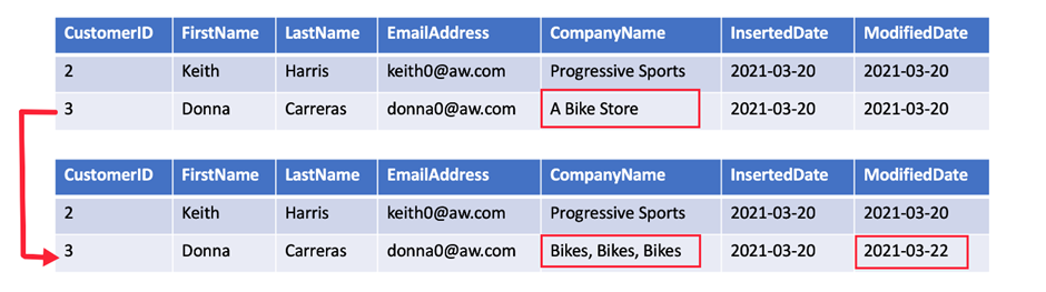
Type 1 SCD:

A Type 1 SCD always reflects the latest values, and when changes in source data are detected, the dimension table data is overwritten. This design approach is common for columns that store supplementary values, like the email address or phone number of a customer. When a customer email address or phone number changes, the dimension table updates the customer row with the new values. It’s as if the customer always had this contact information. The key field, such as CustomerID, would stay the same so the records in the fact table automatically link to the updated customer record.

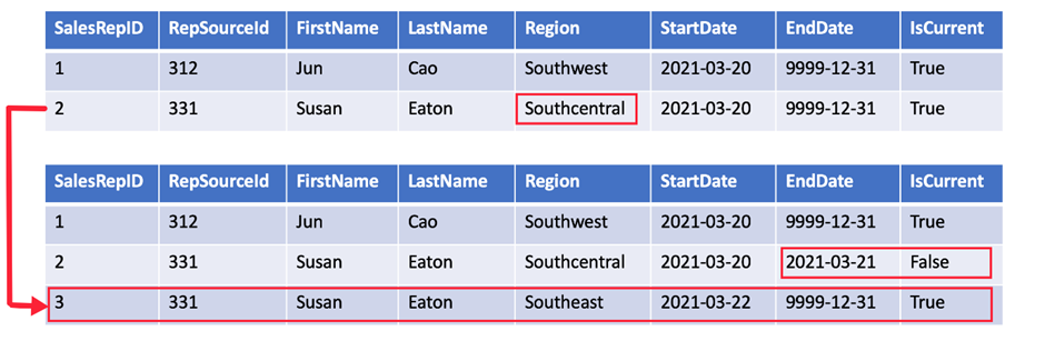
Type 2 SCD:

A Type 2 SCD supports versioning of dimension members. Often the source system doesn’t store versions, so the data warehouse load process detects and manages changes in a dimension table. In this case, the dimension table must use a surrogate key to provide a unique reference to a version of the dimension member. It also includes columns that define the date range validity of the version (for example, StartDate and EndDate) and possibly a flag column (for example, IsCurrent) to easily filter by current dimension members.

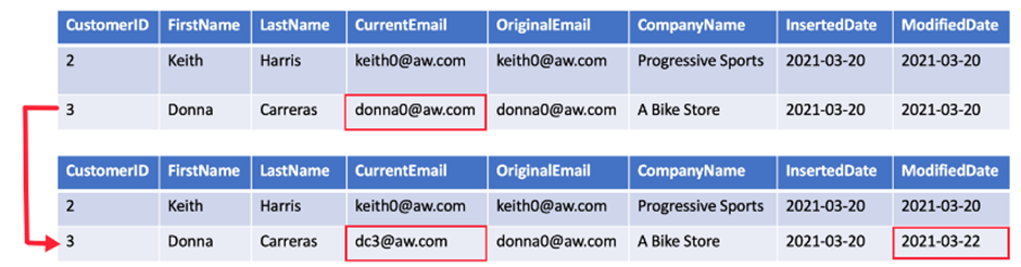
Type 3 SCD:

A Type 3 SCD supports storing two versions of a dimension member as separate columns. The table includes a column for the current value of a member plus either the original or previous value of the member. So Type 3 uses additional columns to track one key instance of history, rather than storing additional rows to track each change like in a Type 2 SCD.

This type of tracking may be used for one or two columns in a dimension table. It is not common to use it for many members of the same table. It is often used in combination with Type 1 or Type 2 members.

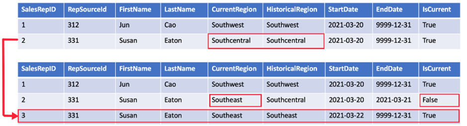
Type 6 SCD:

A Type 6 SCD combines Type 1, 2, and 3. When a change happens to a Type 2 member you create a new row with appropriate StartDate and EndDate. In Type 6 design you also store the current value in all versions of that entity so you can easily report on the current value or the historical value.

Using the sales region example, you split the Region column into CurrentRegion and HistoricalRegion. The CurrentRegion always shows the latest value and the HistoricalRegion shows the region that was valid between the StartDate and EndDate. So for the same salesperson, every record would have the latest region populated in CurrentRegion while HistoricalRegion works exactly like the region field in the Type 2 SCD example.

60.What is the difference between the Mapping data flow and Wrangling data flow transformation activities in Data Factory?

Mapping data flow activity is a visually designed data transformation activity that allows us to design a graphical data transformation logic without the need to be an expert developer, and executed as an activity within the ADF pipeline on an ADF fully managed scaled-out Spark cluster.

Wrangling data flow activity is a code-free data preparation activity that integrates with Power Query Online in order to make the Power Query M functions available for data wrangling using spark execution.

61.When copying data from or to an Azure SQL Database using Data Factory, what is the firewall option that we should enable to allow the Data Factory to access that database?

Allow Azure services and resources to access this server firewall option.

62. Which activity should you use if you need to use the results from running a query?

A look-up activity can give you results from a query or a program. These results can be a single thing, a list of stuff, or something related to how your program works. You can then use these results in another copy data activity.

63. How are the remaining 90 dataset types in Data Factory used for data access?

You can easily use Azure Synapse Analytics, Azure SQL Database, and certain storage accounts for your data in the mapping data flow feature. It also supports Parquet files from blob storage or Data Lake Storage Gen2. However, for data from other sources, you’ll need to first copy it using the Copy activity before you can work with it in a Data Flow activity.

64. Give more details about the Azure Data Factory’s Get Metadata activity

The Azure Data Factory’s “Get Metadata” activity is a fundamental component of Azure Data Factory (ADF) that allows you to retrieve metadata information about various data-related objects within your data factory or linked services. Metadata includes information about datasets, tables, files, folders, or other data-related entities. Here are some key details about the Get Metadata activity:

Purpose:

• Metadata Retrieval: It is used to retrieve metadata information without moving or processing the actual data. This information can be used for control flow decisions, dynamic parameterization, or for designing complex data workflows.

Use Cases:

• Dynamic Execution: You can use the metadata retrieved by this activity to dynamically control which datasets or files to process or copy in subsequent activities.
• Validation: It can be used to check the existence of datasets or files before attempting to use them, ensuring your pipeline only processes existing resources.

Output:

• The Get Metadata activity outputs the metadata as structured JSON data, which includes details like file names, sizes, column names, table schemas, and more, depending on the metadata type and source.

Dynamic Expressions:

• You can use dynamic expressions within the activity configuration to parameterize your metadata retrieval. For example, you can use expressions to construct folder paths or table names at runtime.

In summary, the Get Metadata activity in Azure Data Factory is a powerful tool for gathering information about your data sources and structures, enabling dynamic and data-driven ETL (Extract, Transform, Load) workflows within your data factory pipelines. It helps you make informed decisions and perform data operations based on the state of your data sources.

1. What is Databrics ?

Databricks provides a collaborative and interactive workspace that allows data engineers, data scientists, and analysts to work together on big data projects. It supports various programming languages, including Scala, Python, R, and SQL, making it accessible to a wide range of users.

The platform’s core component is Apache Spark, which enables distributed data processing and analysis across large clusters of computers. Databricks simplifies the deployment and management of Spark clusters, abstracting away much of the underlying infrastructure complexities.

Key features of Databricks include:

Unified Analytics: Databricks offers a collaborative workspace where users can write and execute code, explore data, visualize results, and share insights with their teams.

Apache Spark Integration: Databricks integrates with Apache Spark, providing a high-level interface to manage and scale Spark clusters for big data processing.

Delta Lake: This is an additional feature offered by Databricks, providing a versioned, transactional data lake that improves data reliability and simplifies data management.

Machine Learning: Databricks supports building and deploying machine learning models using popular libraries like MLlib, Scikit-learn, and TensorFlow.

Data Integration: Databricks can connect to various data sources, such as data lakes, databases, and data warehouses, allowing users to analyze and process data from multiple sources.

Job Scheduling: Users can schedule and automate data processing jobs, making it easier to run repetitive tasks at specific times or intervals.

Security and Collaboration: Databricks provides role-based access control and allows teams to collaborate securely on projects.

2. What is the difference between Databrics and Data factory?

In simple terms, Databricks is a platform for big data analysis and machine learning, while Data Factory is a cloud-based service used for data integration, movement, and orchestration. Databricks is more suitable for data analysis and advanced analytics tasks, while Data Factory is ideal for data movement and transformation between different data sources and destinations.

3. Describe Spark Architecture.

The architecture of an Apache Spark application is based on a distributed computing model that allows it to process large-scale data across multiple nodes in a cluster. Spark applications are designed to be fault-tolerant, scalable, and efficient. Here’s an overview of the key components and the flow of data in a typical Apache Spark application:

1. Driver Program:

• The Driver Program is the entry point of a Spark application. It runs on the master node and is responsible for creating the SparkContext, which is the entry point to any Spark functionality.
• The Driver Program defines the high-level control flow of the application, including tasks, stages, and dependencies between transformations and actions.

2. SparkContext (SC):

• SparkContext is the entry point to any Spark functionality. It establishes a connection to the cluster manager (e.g., YARN, Mesos, or Spark’s standalone cluster manager) to acquire resources for the application.
• The SparkContext coordinates with the Cluster Manager to allocate and manage executors across the worker nodes.

3. Cluster Manager:

• The Cluster Manager is responsible for managing the resources across the cluster, allocating tasks to workers, and ensuring fault tolerance.
• It can be YARN, Mesos, or Spark’s standalone cluster manager.

4. Worker Nodes:

• Worker Nodes are the machines in the cluster where actual data processing takes place.
• Each worker node hosts one or more executors, which are separate JVM processes responsible for executing tasks.

5. Executors:

• Executors are processes on the worker nodes responsible for executing individual tasks and storing data in memory or disk storage.
• They manage the data that is cached and reused across multiple Spark operations, reducing the need to read data from disk repeatedly.

6. Resilient Distributed Dataset (RDD):

• RDD is the fundamental data abstraction in Spark. It represents an immutable, fault-tolerant collection of objects that can be processed in parallel.
• RDDs are divided into partitions, and each partition is processed on a separate executor.

7. Transformations:

• Transformations are operations on RDDs that create new RDDs from existing ones. Examples include map, filter, reduceByKey, etc.
• Transformations are lazily evaluated, meaning they are not executed until an action is called.

8. Actions:

• Actions are operations that trigger the execution of transformations and return results to the Driver Program or write data to external storage.
• Examples of actions include collect, count, save, etc.
• Actions trigger the actual computation and materialize the RDD lineage.

9. Lineage Graph (DAG):

• Spark constructs a Directed Acyclic Graph (DAG) of the transformations (logical execution plan) and optimizes it before execution to minimize data shuffling and improve performance.

10. Data Sources and Sinks:

• Spark applications can read data from various sources (e.g., HDFS, S3, databases) and write data to external storage systems (e.g., HDFS, databases, file systems).

The architecture of Spark allows it to distribute data and computation across the cluster efficiently, providing fault tolerance, data locality, and high-performance data processing.

4. What is the maximum size of worker node you have used?

Storage 64 GB worker node.

Note – If you say more than that in interview garbage in and out problem occur so strict to max 64 GB.

5. How do you choose cluster configuration in Databrics?

• For normal ETL/ELT work – Memory optimize
• Quick Dev test – General Purpose
• For Shuffle intensive work(e.g lot many join) – Storage optimize

6. What is the difference between repartition and coalesce?

Both repartition and coalesce are Spark transformations used to control the distribution of data across partitions in a DataFrame or an RDD (Resilient Distributed Dataset). They affect how data is physically stored and distributed across the nodes of a cluster.

In summary, the key differences are:

• repartition can increase or decrease the number of partitions and performs a full data shuffle, while coalesce only reduces the number of partitions and tries to minimize data movement.
• Use repartition when you need to achieve a specific number of partitions or evenly distribute data for better parallelism. Use coalesce when you want to reduce the number of partitions efficiently without triggering a full shuffle.

# For DataFrame repartition
df.repartition(numPartitions)
# For DataFrame coalesce
df.coalesce(numPartitions)

7. What is the drawback of coalesce?

The coalesce transformation in Spark is a powerful tool to reduce the number of partitions in a DataFrame or RDD without a full shuffle, which can be beneficial for certain use cases. However, it also has some drawbacks that you should be aware of:

Data Skew:

• When reducing the number of partitions with coalesce, Spark tries to minimize data movement and merges partitions into a smaller number of partitions. This approach can lead to data skew, where some partitions may end up with significantly more data than others.
• Data skew can negatively impact performance since a few partitions may become “hotspots” that are processed much slower than others, leading to inefficient resource utilization.

Uneven Data Distribution:

• Similar to data skew, coalesce can result in uneven data distribution across the reduced partitions. If the data has an uneven distribution or if certain keys have significantly more data than others, this can lead to suboptimal performance for subsequent operations like joins or aggregations.

Limited to Reduce Partitions:

• Unlike repartition, which allows you to increase or decrease the number of partitions, coalesce can only reduce the number of partitions. You cannot use coalesce to increase the number of partitions, which might be needed for certain operations that benefit from increased parallelism.

Less Parallelism:

• By reducing the number of partitions, you may reduce the level of parallelism in subsequent processing. This can lead to underutilization of resources, particularly if you have a large cluster with many available cores.

Optimal Partition Size:

• Choosing the right number of partitions for coalesce is crucial. If you set the number of partitions too low, you might end up with partitions that are too large to fit into memory, leading to performance issues.

8. If we have .gz file, how are they distributed in the spark

No, it will not be distributed, it will be single threaded.

9. What is the difference between “from pyspark.sql.type import *” and from pyspark.sql.types import xyz ?

Performance.

If we write from pyspark.sql.type import * every library under sql will get imported which will affect the performance.

10. What is the default partition size?

11. Have you worked on Databrics SQL? What is it all about?

Databrics SQL provides a simple experience for SQL users who wants to run quick ad-hoc queries on their data lake, create multiple visualization type to explore query result from different perspectives, and build and share dashboards.

12. What are the SQL endpoints? How are they different from cluster?

SQL endpoints in Databricks are secure entry points that allow users to execute SQL queries against their data. They provide a familiar SQL interface for querying and analyzing data stored in Databricks tables or external data sources like Delta Lake or Apache Spark tables.

Difference from cluster:

• A cluster in Databricks is a set of computing resources (e.g., virtual machines) used to run data processing and analytics workloads, such as Spark jobs and notebooks.
• SQL endpoints, on the other hand, are query interfaces specifically designed for executing SQL queries against data without the need to start a separate cluster.
• While clusters are general-purpose compute resources for various data processing tasks, SQL endpoints focus specifically on SQL query execution and can handle multiple concurrent queries efficiently.

13. What do you mean by interactive and job cluster?

Interactive Cluster: An interactive cluster in Databricks is designed for interactive data exploration and analysis. It provides a collaborative workspace where users can run notebooks and execute code interactively. Interactive clusters allow users to iteratively explore data, visualize results, and experiment with different analyses in a shared environment.

Job Cluster: A job cluster in Databricks is used for running batch jobs and automated data processing tasks. Unlike interactive clusters, job clusters are not continuously running and are launched on-demand to execute specific jobs at scheduled intervals or upon request. Job clusters are ideal for running ETL (Extract, Transform, Load) workflows, machine learning training, and other automated data processing tasks.

14. What is Auto scaling in databrics cluster?

• Auto Scaling in Databricks cluster automatically adjusts the cluster resources (number of worker nodes) based on workload demand, optimizing resource utilization and cost efficiency.
• Users can configure the Auto Scaling behaviour, setting minimum and maximum limits for the number of worker nodes and defining scaling policies based on metrics like CPU utilization or memory usage.

15. What is Managed and unmanaged tables in databrics?

In Databricks, managed and unmanaged tables are two different ways of organizing and managing data in the Databricks Delta Lake or Apache Spark table format:

Managed Tables:

• Managed tables, also known as Delta tables, are tables whose metadata and data files are managed and controlled by Databricks.
• When you create a managed table, Databricks handles the storage, organization, and cleanup of data files and metadata automatically.
• This means that when you delete a managed table, Databricks will also delete all the associated data files from storage.
• Managed tables are easy to work with since Databricks takes care of most of the underlying management tasks.

Unmanaged Tables:

• Unmanaged tables are tables where you have direct control over the data files, and Databricks does not manage the data or metadata.
• When you create an unmanaged table, you need to specify the data files’ location, and Databricks relies on you to handle file organization and cleanup.
• If you delete an unmanaged table, Databricks only removes the metadata, but the data files remain intact in the specified location.
• Unmanaged tables provide more control over the data, making them suitable for scenarios where you have existing data files in a specific location.

In summary, managed tables are automatically managed by Databricks, including data file storage and cleanup, while unmanaged tables require you to handle the data files’ management and organization manually.

16. How do you configure numbers of core in worker?

Generally, Number of cores = Numbers of partitions.

17. How do you handle BAD records in databrics?

There are two ways to handle errors in databrics:

MODE:

1. Permissive(Error value will be stored as null and entire error row will be saved as column)
2. Dropmalformed (Whole records that has error values will get drop off)
3. Failfast(When error is recognized execution stops)

BAD RECORD PATH (Redirect value to separate path)

18. Given a list of json string, count the number of IP address, order of output does not matter?

To count the number of unique IP addresses from a list of JSON strings, you can follow these steps

1. Parse the JSON strings and extract the IP addresses.
2. Use a set to store the unique IP addresses.
3. Count the number of elements in the set, which will give you the count of unique IP addresses.

Here’s the Python code to achieve this:

Output:

19. What is difference between narrow and wide transformation?

In Databricks (and Apache Spark), transformations are operations performed on a distributed dataset (RDD or DataFrame). These transformations are broadly classified into two categories: narrow transformations and wide transformations.

1. Narrow Transformations:

• Narrow transformations are transformations where each input partition contributes to at most one output partition.
• These transformations do not require data to be shuffled across the partitions, and they can be performed in parallel on each partition independently.
• Examples of narrow transformations include `map`, `filter`, and `union`.

2. Wide Transformations:

• Wide transformations are transformations where each input partition can contribute to multiple output partitions.
• These transformations require data to be shuffled and redistributed across the partitions, which involves a data exchange between the worker nodes.
• Wide transformations usually result in a stage boundary, which involves a physical data exchange and a shuffle operation.
• Examples of wide transformations include `groupBy`, `join`, and `sortByKey` (for RDDs).

The main difference between narrow and wide transformations lies in how they handle data distribution and shuffling. Narrow transformations can be executed efficiently in a parallel and distributed manner without the need for shuffling data between partitions. On the other hand, wide transformations require a data shuffle, which can be a more expensive operation as it involves network communication and data redistribution.

To optimize Spark job performance, it’s essential to minimize the usage of wide transformations and use them judiciously. When designing data processing pipelines, try to keep as many transformations as possible as narrow transformations to reduce data shuffling and improve execution efficiency.

20. What is shuffle? why shuffle occur? What causes the shuffle?

In the context of Apache Spark (and Databricks), a “shuffle” refers to the process of redistributing data across partitions in a distributed computing environment. Shuffle occurs when data needs to be rearranged to satisfy a specific operation, such as aggregations, joins, or sorting, where data from multiple partitions needs to be brought together to perform the operation effectively.

Shuffle occurs for the following reasons:

1. Data Reorganization for Operations:

• Certain operations, like grouping elements by a key in a `groupBy` or performing a `join` between two datasets, require data with the same keys to be brought together into the same partition to perform the operation.
• For example, when you perform a `groupBy` on a DataFrame or RDD based on a particular column, Spark needs to gather all the rows with the same key from various partitions and organize them together.

2. Data Skew:

• Data skew occurs when the distribution of data across partitions is uneven, causing some partitions to have significantly more data than others.
• In scenarios with data skew, a few partitions can become overloaded with data, leading to slower processing times for those partitions and suboptimal resource utilization.
• To handle data skew, Spark may need to redistribute data through shuffle to achieve a more balanced data distribution across partitions.

3. Performance Optimization:

• In some cases, shuffle can be used to optimize performance by co-locating related data on the same partitions, reducing the amount of data exchange during certain operations.
• For example, Spark can leverage shuffle to bring together data that will be accessed together, reducing the need to read data from various partitions separately.

It’s essential to be aware of the cost of shuffle operations since they involve data movement across the network, which can be expensive in terms of computation and time. Minimizing shuffle whenever possible is a key performance consideration when designing and optimizing Apache Spark or Databricks jobs. Proper partitioning of data and careful selection of appropriate operations can help reduce the frequency and impact of shuffling.

21. What is difference between sortBy and OrderBy?

We can use either sort() or Orderby() built in function to sort a particular dataframe in a ascending or descending order over at least one column.

Sort()

Sort() method will sort() the records in each partition and then return the final output which means that the order of the output data is not guaranteed because data is ordered on partition level but your data frame may have thousands of partitions distributed across the cluster.

Since the data is not collected into a single executor the sort() method is efficient thus more suitable  when sorting is not critical for your use case.

Orderby()

Unlike Sort(), the orderBy() function guarantee a total order in the output. This happen because the data will be collected into a single executor in order to be sorted.

This means that orderBy() is more inefficient compared to sort()

22. What is difference between map and map partition?

map()

map is a transformation that applies a function to each element of the RDD or DataFrame, processing the elements one at a time. whatever transformation you mentation on the data. It has a one-to-one mapping between input and output elements.

mapPartitions()

mapPartitions is a transformation that applies a function to each partition of the RDD or DataFrame, processing multiple elements within each partition at once. It has a one-to-many mapping between input partitions and output partitions.

In summary, map processes data element-wise, while mapPartitions processes data partition-wise, which can lead to more efficient data processing when dealing with expensive operations or when you need to maintain some state across multiple elements within a partition.

23. What is lazy evaluation in spark?

Lazy evaluation in Spark refers to the evaluation strategy where transformations on RDDs (Resilient Distributed Datasets) or DataFrames are not executed immediately when called. Instead, Spark builds up a logical execution plan (DAG – Directed Acyclic Graph) representing the sequence of transformations. The actual execution is deferred until an action is called.

Key points about lazy evaluation in Spark:

Transformations are Deferred:

When you apply a transformation on an RDD or DataFrame (e.g., `map`, `filter`, `groupBy`, etc.), Spark does not perform the actual computation right away. Instead, it records the transformation in the execution plan.

Logical Execution Plan (DAG):

Spark builds a directed acyclic graph (DAG) that represents the series of transformations in the order they were applied. Each node in the DAG represents a transformation, and the edges represent data dependencies.

Efficient Optimization:

Since Spark has access to the entire transformation sequence before executing any action, it can optimize the execution plan for performance, by combining and reordering transformations to reduce data shuffling and improve parallelism.

Lazy Execution with Actions:

Spark only performs the actual computation when an action is called (e.g., `collect`, `count`, `save`, etc.). Actions trigger the execution of the entire DAG of transformations, starting from the original RDD or DataFrame.

Benefits of lazy evaluation:

• It allows Spark to optimize the execution plan before actually running the job, leading to more efficient data processing.
• Lazy evaluation reduces unnecessary computation and data shuffling, as Spark can skip intermediate transformations that are not needed to compute the final result.
• It provides an opportunity for developers to chain multiple transformations together before triggering the actual computation, which can lead to more concise and modular code.

Overall, lazy evaluation is a fundamental optimization technique in Spark that improves performance by deferring the execution of transformations until the results are required.

24. What are the different levels of persistence in spark?

In Apache Spark, persistence (also known as caching) is a technique to store intermediate or final computation results in memory or disk. By persisting data, Spark can reuse it across multiple Spark operations without re-computing it from the original data source. This can significantly improve the performance of iterative algorithms or when the same data is accessed multiple times.

There are different levels of persistence available in Spark:

1. MEMORY_ONLY (or MEMORY_ONLY_SER):

• This is the simplest level of persistence, where the RDD or DataFrame is stored in memory as deserialized Java objects (MEMORY_ONLY) or serialized bytes (MEMORY_ONLY_SER).
• MEMORY_ONLY is suitable when the data fits comfortably in memory and can be quickly accessed without deserialization overhead.
• MEMORY_ONLY_SER is useful when the data size is larger than the available memory, as it saves memory space by keeping the data in a serialized format.

2. MEMORY_AND_DISK:

• In this level of persistence, if an RDD or DataFrame does not fit entirely in memory, Spark spills the excess partitions to disk while keeping the remaining partitions in memory.
• MEMORY_AND_DISK provides a balance between in-memory access speed and disk space utilization. However, accessing data from disk is slower than accessing it from memory, so it may lead to performance degradation for frequently accessed data that spills to disk.

3. MEMORY_AND_DISK_SER:

• Similar to MEMORY_AND_DISK, but it stores data in serialized format to save memory space.
• MEMORY_AND_DISK_SER can be beneficial when the dataset is large and cannot fit entirely in memory.

4. DISK_ONLY:

• In this level of persistence, data is stored only on disk and not kept in memory.
• DISK_ONLY is suitable when memory is limited, and the data size is much larger than the available memory.
• Accessing data from disk is slower than accessing it from memory, so performance might be affected.

5. OFF_HEAP:

• This is an experimental feature in Spark that stores data off-heap (outside the JVM heap space).
• OFF_HEAP is useful for very large datasets that require a significant amount of memory, as it can help avoid Java garbage collection overhead.

Each persistence level offers different trade-offs between memory utilization and access speed. The choice of persistence level depends on factors like the size of data, available memory, and the frequency of data access in your Spark application. Properly selecting the persistence level can greatly impact the overall performance and efficiency of Spark jobs.

Import org.apache.spark.storage.storagelevel
Val rdd2 = rdd.persist(StorageLevel.MEMORY_ONLY)

25. How to check data skewness of how many rows present in each partition?

26. What are the different planes in Databrics?

In cloud computing and distributed systems, the concept of “planes” is used to categorize different aspects of the system’s architecture and management. The three main planes are:

Data Plane:

• The Data Plane is responsible for handling and processing the actual user data and performing the intended operations on the data.
• In Databricks, the Data Plane is where data processing tasks take place, such as executing Spark jobs, running notebooks, and performing data transformations.

Control Plane:

• The Control Plane is responsible for managing and coordinating the overall system’s operation and behavior.
• In Databricks, the Control Plane manages the cluster lifecycle, monitors resource allocation, schedules jobs, and handles administrative tasks such as authentication, access control, and cluster management.

Management Plane:

• The Management Plane provides tools and interfaces for users and administrators to configure, monitor, and manage the system and its components.
• In Databricks, the Management Plane includes the Databricks Workspace, which provides a collaborative environment for managing notebooks, libraries, dashboards, and other resources.

Each plane plays a crucial role in the operation and management of cloud-based distributed systems like Databricks, helping to separate concerns and provide a clear and organized way to design and manage complex systems.

27. How to drop duplicate from following dataframe?

STATION_ID	DATE_CHANGED  STATION_ID
1	6/7/2006 6:00
1	9/26/2000 6:00
2	7/29/2005 6:00
2	6/6/2001 6:00
4	6/8/2001 6:00
4	11/25/2003 7:00
7	6/12/2001 6:00
8	6/4/2001 6:00
8	4/3/2017 18:36

df.sort_values('DATE_CHANGED').drop_duplicates('STATION_ID',keep='last')

28. How to improve performance of a notebook in databrics?

To improve notebook performance in Databricks, you can follow these best practices and optimization techniques:

1. Cluster Configuration: Use an appropriately sized cluster based on your workload. Scaling up the cluster can significantly improve performance, especially for resource-intensive tasks. Databricks provides various cluster types with different CPU, memory, and GPU configurations. You can monitor cluster performance to identify bottlenecks.

 2. Autoscaling: Enable autoscaling to automatically adjust the number of workers based on the workload. This helps optimize resource allocation and reduce costs during idle periods.

 3. Caching and Persistence: Utilize caching and persistence to store intermediate results or dataframes that are frequently accessed. This can speed up subsequent operations by avoiding redundant computations.

 4. Optimize Data Format: Choose appropriate data formats to store and read data. For example, using Parquet format for storage is more efficient than using CSV or JSON due to its columnar storage and compression capabilities.

5. Limit Data Shuffling: Minimize data shuffling as it can be a resource-intensive operation. Data shuffling occurs when the data needs to be redistributed across partitions, and it can impact performance significantly.

 6. Tune Spark Configurations: Adjust Spark configurations like `spark.sql.shuffle.partitions`, `spark.executor.memory`, and `spark.driver.memory` to optimize performance based on your specific workload and data size.

7. Use Delta Lake: If possible, leverage Delta Lake for transactional and versioned data storage. It offers significant performance improvements for analytics workloads.

 8. Spark UI Optimization: Use the Spark UI to monitor job progress, identify performance bottlenecks, and optimize query plans. Look for stages with long execution times or high shuffle data, and try to optimize them.

 9. Use Databricks Runtime: Databricks Runtime is optimized by default and includes various performance improvements. Always use the latest stable version for the best performance and new features.

 10. Notebook Code Optimization: Review and optimize your notebook code regularly. Avoid unnecessary data transformations and use efficient Spark APIs and DataFrame operations when possible.

 11. Resource Management: Be mindful of resource utilization in notebooks. Avoid running multiple long-running notebooks simultaneously to prevent resource contention.

 12. Data Pruning: For large datasets, consider pruning the data to limit the amount of data processed, especially if you only need a specific time range or subset of data.13. External Data Cache: Use the Databricks External Data Cache to cache data across multiple notebooks or clusters, reducing data transfer time and computation overhead.

Remember that the effectiveness of these optimizations depends on your specific use case and data, so it’s essential to monitor and fine-tune your configurations regularly to achieve the best performance.

29. How to pass parameter though parent notebook in the child notebook?

In Databricks, you can pass parameters from a parent notebook to a child notebook using the dbutils.notebook.run function. This function allows you to call a child notebook and pass parameters as input to the child notebook. Here’s a step-by-step guide on how to do this.

Step 1: Define the Parent Notebook:

In the parent notebook, you can define the parameters you want to pass to the child notebook and then call the child notebook using the dbutils.notebook.run function.

# Parent Notebook

param1 = "value1"
param2 = 42

dbutils.notebook.run("ChildNotebook", 0, {"param1": param1, "param2": param2})

Step 2: Access Parameters in the Child Notebook:

In the child notebook, you can access the parameters passed from the parent notebook using the dbutils.widgets module. You need to define widgets with the same names as the parameters used in the parent notebook.

# ChildNotebook

param1 = dbutils.widgets.get("param1")
param2 = dbutils.widgets.get("param2")

print("Received parameters in child notebook:")
print("param1:", param1)
print("param2:", param2)

By using the dbutils.widgets.get function with the same name as the parameter, you can retrieve the values passed from the parent notebook.

30. What are the dbutils function available in databrics?

In Databricks, the `dbutils` module provides utility functions that help you interact with the Databricks environment, access files, manage libraries, and more. These functions are designed to simplify common tasks when working with Databricks notebooks and clusters. Here are some of the commonly used `dbutils` functions available in Databricks:

1. File System Operations:

•    dbutils.fs.ls(path): List files in a directory.
•    dbutils.fs.cp(source, destination): Copy a file or directory.
•    dbutils.fs.mv(source, destination): Move or rename a file or directory.
•    dbutils.fs.rm(path, recurse=True): Remove a file or directory.
•    dbutils.fs.mkdirs(path): Create directories recursively.

2. Notebook Utilities:

   – `dbutils.notebook.run(notebook_path, timeout_seconds, arguments)`: Run a different notebook and pass parameters.
   – `dbutils.notebook.exit(result)`: Stop execution of the current notebook and return a result.

3. Widgets:
   – dbutils.widgets.text(name, defaultValue): Create a text widget.
   – dbutils.widgets.get(name): Get the value of a widget.
   – dbutils.widgets.dropdown (name, defaultValue, choices): Create a dropdown widget.
   – dbutils.widgets.combobox (name, defaultValue, choices): Create a combo box widget.
   – dbutils.widgets.multiselect (name, defaultValue, choices): Create a multiselect widget.

 4. Library Management:
   – dbutils.library.install (pypi_package): Install a PyPI package as a library.
   – dbutils.library.restartPython(): Restart the Python interpreter to apply library changes.
   – dbutils.library.remove (library_path): Remove a library.

 5. Secret Management:
   – dbutils.secrets.get(scope, key): Retrieve a secret from the Databricks Secret Manager.

 6. Azure Blob Storage Utilities:
   – dbutils.fs.mount(source, mount_point): Mount an Azure Blob Storage container.
   – dbutils.fs.unmount(mount_point): Unmount an Azure Blob Storage container.

31. What is broadcast join?

In Databricks, a broadcast join is a type of join operation used in Spark SQL that optimizes the performance of joining a small DataFrame (or table) with a larger DataFrame (or table). It is based on the concept of broadcasting the smaller DataFrame to all the nodes of the cluster, allowing each node to perform the join locally without shuffling the data. This approach is beneficial when one of the DataFrames is small enough to fit in memory and the other DataFrame is significantly larger.

When performing a broadcast join, Spark automatically broadcasts the smaller DataFrame to all the worker nodes in the cluster, making it available in memory. Then, the worker nodes use this broadcasted copy to perform the join locally with their respective partitions of the larger DataFrame. By doing so, Spark can avoid costly shuffling operations, which can lead to significant performance improvements.

To leverage the benefits of a broadcast join in Spark SQL, you can explicitly hint the optimizer to use it for a specific join by using the BROADCAST keyword. For example:

By adding the /*+ BROADCAST(small_df) */ hint to the SQL query, you inform Spark to use a broadcast join for the specified small_df DataFrame.

32. What is struct function?

In Databricks, the struct function is a Spark SQL function used to create a new struct column by combining multiple columns together. A struct column is similar to a struct or namedtuple in programming languages, allowing you to group multiple values together into a single column. This is especially useful when you want to create complex data types or nest multiple fields within a single DataFrame column.

The struct function takes multiple column expressions as arguments and returns a new column containing the combined values as a struct. Each input column becomes a field within the resulting struct column. The struct columns can then be used like any other DataFrame column, allowing you to access nested data in a structured manner.

Here’s the basic syntax of the struct function:

• column1, column2, …, columnN: The input columns that you want to combine into the struct column.

Here’s a practical example of using the struct function:

Output look like this:

33. What is explode function does?

In Databricks, the explode function is a Spark SQL function used to transform an array or map column into multiple rows, effectively “exploding” the elements of the array or map into separate rows. This is particularly useful when you have data with nested arrays or maps, and you want to flatten the structure to perform operations on individual elements.

The explode function works on columns that contain arrays or maps and produces a new DataFrame with each element of the array or map expanded into separate rows. For arrays, each element of the array becomes a separate row, and for maps, the key-value pairs of the map become separate rows.

Here’s the basic syntax of the explode function:

• column: The column containing the array or map that you want to explode.
• alias: An optional alias to give a name to the resulting column after the explosion.

Let’s look at a practical example using the explode function:

The output will look like:

As you can see, the fruits array column is exploded into separate rows, where each fruit from the array becomes an individual row in the resulting DataFrame.

The explode function is a powerful tool when working with nested data structures, and it allows you to perform operations on individual elements within arrays or maps efficiently in Databricks. It can be combined with other Spark SQL functions to perform complex data manipulations on nested data.

34. Is it possible to combine Databricks and Azure Notebooks?

They operate similarly, but data transfer to the cluster requires manual coding. This Integration is now easily possible thanks to Databricks Connect. On behalf of Jupyter, Databricks makes a number of improvements that are specific to Databricks.

35. What exactly does caching entail?

Temporary holding is referred to as the cache. The process of temporarily storing information is referred to as caching. You’ll save time and lessen the load on the server when you come back to a frequently visited website because the browser will retrieve the data from the cache rather than from the server.

36. What are the different types of caching are there?

There are four types of caching that stand out:

• Information caching
• Web page caching
• Widespread caching
• Output or application caching.

37. Should you ever remove and clean up any leftover Data Frames?

Cleaning Frames is not necessary unless you use cache(), which will use a lot of network bandwidth. You should probably clean up any large datasets that are being cached but aren’t being used.

38. What different ETL operations does Azure Databricks carry out on data?

The various ETL processes carried out on data in Azure Databricks are listed below:

• The data is converted from Databricks to the data warehouse.
• Bold storage is used to load the data.
• Data is temporarily stored using bold storage

39. Does Azure Key Vault work well as a substitute for Secret Scopes?

That is certainly doable. However, some setup is necessary. The preferred approach is this. Instead of changing the defined secret, start creating a scoped password that Azure Key Vault will backup if the data in secret needs to be changed.

40. How should Databricks code be handled when using TFS or Git for collaborative projects?

TFS is not supported, to start. Your only choices are dispersed Git repository systems and Git. Although it would be ideal to integrate Databricks with the Git directory of notebooks, it works much like a different project clone. Making a notebook, trying to commit it to version control, and afterwards updating it are the first steps.

41. Does Databricks have to be run on a public cloud like AWS or Azure, or can it also run on cloud infrastructure?

This is not true. The only options you have right now are AWS and Azure. But Databricks uses Spark, which is open-source. Although you could build your own cluster and run it in a private cloud, you’d be giving up access to Databricks’ robust features and administration.

42. How is a Databricks personal access token created?

• On the Databricks desktop, click the “user profile” icon in the top right corner.
• Choosing “User setting.”
• Activate the “Access Tokens” tab.
• A “Generate New Token” button will then show up. Just click it.

43. Is code reuse possible in the Azure notebook?

We should import the code first from Azure notebook into our notebook so that we can reuse it. There are two ways we can import it.

• We must first create a component for the code if it is located on a different workstation before integrating it into the module.
• We can import and use the code right away if it is on the same workstation.

44. What is a Databricks cluster?

The settings and computing power that make up a Databricks cluster allow us to perform statistical science, big data, and powerful analytic tasks like production ETL, workflows, deep learning, and stream processing.

45. Is databrics provide database services, if no then where it saves the delta table?

Azure Databricks does not directly provide traditional database services like SQL Server or Azure SQL Database. Instead, it is an Apache Spark-based analytics platform designed to process and analyze big data workloads. However, it can work with various data sources and databases to perform data processing and analytics tasks.

One of the popular data storage options in Azure Databricks is Delta Lake, which is an open-source storage layer that brings ACID (Atomicity, Consistency, Isolation, Durability) transactions to data lakes. Delta Lake provides some database-like functionalities on top of cloud storage systems like Azure Data Lake Storage or Azure Blob Storage.

When you save a Delta table in Azure Databricks, the data is typically stored in your specified cloud storage (e.g., Azure Data Lake Storage or Azure Blob Storage). Delta Lake keeps track of the changes made to the data, allowing for versioning and transactional capabilities.

46. Is Databricks only available in the cloud and does not have an on-premises option?

Yes. Databricks’ foundational software, Apache Spark, was made available as an on-premises solution, allowing internal engineers to manage both the data and the application locally. Users who access Databricks with data on local servers will encounter network problems because it is a cloud-native application. The on-premises choices for Databricks are also weighed against workflow inefficiencies and inconsistent data.

47. In Parameter what does it mean by inferSchema as True

In the context of data processing frameworks like Apache Spark and PySpark (used in Azure Databricks), the inferSchema parameter is used when reading data from external sources like CSV, JSON, Parquet, etc. It is a configuration option that determines whether Spark should automatically infer the data types of the columns in the DataFrame based on the data content.

When inferSchema is set to True, Spark will automatically examine a sample of the data to infer the data types for each column. This process involves analyzing the data values in each column and making educated guesses about the appropriate data types. For example, if a column predominantly contains numeric values, Spark might infer it as an integer or a double data type. Similarly, if a column primarily contains strings, it might infer it as a string data type.

Setting inferSchema to True can be convenient and save time, especially when working with large datasets with many columns. Spark’s ability to automatically infer data types allows you to read data without explicitly specifying the schema, making the code shorter and more flexible.

However, it’s essential to be cautious when using inferSchema, as it relies on a sample of the data and might not always make accurate decisions, especially when the data is sparse or there are outliers. In such cases, it’s recommended to provide an explicit schema to ensure the correct data types are used.

48. What are the difference between Auto Loader vs COPY INTO?

Auto Loader:

Auto Loader incrementally and efficiently processes new data files as they arrive in cloud storage without any additional setup. Auto Loader provides a new Structured Streaming source called cloudFiles. Given an input directory path on the cloud file storage, the cloudFiles source automatically processes new files as they arrive, with the option of also processing existing files in that directory.

When to use Auto Loader instead of the COPY INTO?

• If you’re going to ingest files in the order of thousands, you can use COPY INTO. If you are expecting files in the order of millions or more over time, use Auto Loader. Auto Loader requires fewer total operations to discover files compared to COPY INTO and can split the processing into multiple batches, meaning that Auto Loader is less expensive and more efficient at scale.
• If your data schema is going to evolve frequently, Auto Loader provides better primitives around schema inference and evolution. See Configure schema inference and evolution in Auto Loader for more details.
• Loading a subset of re-uploaded files can be a bit easier to manage with COPY INTO. With Auto Loader, it’s harder to reprocess a select subset of files. However, you can use COPY INTO to reload the subset of files while an Auto Loader stream is running simultaneously.

spark.readStream.format("cloudfiles") # Returns a stream data source, reads data as   it arrives based on the trigger.

.option("cloudfiles.format","csv") # Format of the incoming files
.option("cloudfiles.schemalocation", "dbfs:/location/checkpoint/")  The location to store the inferred schema and subsequent changes

.load(data_source)
.writeStream.option("checkpointlocation","dbfs:/location/checkpoint/") # The location of the stream’s checkpoint

.option("mergeSchema", "true") # Infer the schema across multiple files and to merge the schema of each file. Enabled by default for Auto Loader when inferring the schema.

.table(table_name)) # target table

49. How to do partition data in the databrics?

Partitioning data in Databricks, or any other data processing platform, can greatly improve query performance and overall data organization. Partitioning involves dividing your data into smaller, more manageable parts based on specific criteria, such as a particular column’s values. This helps reduce the amount of data that needs to be scanned when executing queries, leading to faster query execution times. Here’s how you can partition data in Databricks:

1. Choose a Partition Column: Select a column in your dataset that you want to use for partitioning. Common choices are date columns, country codes, or any other attribute that can be used to logically group your data.

2. Organize Data: Arrange your data in the storage system (like a data lake) in a way that reflects the partitioning scheme you’ve chosen. This usually involves creating subdirectories for each partition, where the name of the subdirectory corresponds to the partition key’s value. For example, if you’re partitioning by year and month, your directory structure might look like:

3. Write Partitioned Data: When writing data into Databricks, make sure to specify the partition column and value appropriately. Databricks has integrations with various data sources like Parquet, Delta Lake, and more, which support partitioning.

For example, if you’re using Apache Spark to write partitioned Parquet data, you can do something like this:

4. Querying Partitioned Data: When querying partitioned data, Databricks and Spark will automatically take advantage of the partitioning scheme to optimize query performance. You can filter your queries based on the partition column, and Spark will only scan the relevant partitions, reducing the amount of data scanned.

50. How to rename a column name in dataframe?

51. If we have an employee data frame and we want to add 1000 to those employee’s salary who have a more than 10,000 salary how to do that?

You can achieve this using PySpark by applying a transformation to the DataFrame to update the salary values based on a condition. Here’s a sample code to add 1000 to the salary of employees who have a salary greater than 10,000:

Update using multiple conditions.

52. What is surrogate key in database concept?

A surrogate key is a unique identifier that is added to a database table to serve as a primary key. Unlike natural keys, which are based on existing data attributes (such as names, dates, or other real-world information), surrogate keys are typically artificially created and have no inherent meaning. They are used primarily to improve the efficiency and performance of database operations.

Surrogate keys offer several benefits:

1. Uniqueness: Surrogate keys are generated in a way that ensures their uniqueness across the entire table. This eliminates the risk of duplicate entries that might occur with natural keys.

2. Stability: Since surrogate keys are not based on changing attributes like names or addresses, they remain stable over time. This makes them ideal for linking data and maintaining relationships even when other attributes change.

3. Performance: Surrogate keys can improve database performance by making indexes and joins more efficient. They tend to be shorter than meaningful attributes, leading to faster data retrieval and better query performance.

4. Data Privacy: Surrogate keys help maintain data privacy by not exposing sensitive or personal information in the key itself. This can be important for compliance with data protection regulations.

5. Simplifying Joins: When tables are linked through relationships, using surrogate keys can simplify the process of joining tables, as the keys are consistent and predictable.

6. Data Warehousing: In data warehousing scenarios, surrogate keys are often used to create fact and dimension tables, facilitating efficient reporting and analysis.

An example of a surrogate key might be an auto-incrementing integer that is assigned to each new record added to a table. This key is unique and has no inherent meaning, making it an ideal primary key for efficient database operations.

It’s worth noting that while surrogate keys offer various advantages, there are cases where natural keys (based on meaningful attributes) might be more appropriate, especially when the data itself carries important semantic meaning. The choice between surrogate and natural keys depends on the specific requirements of the database schema and the overall data model.

53. If I have a dataframe called student where I have Name, email, department and activity date columns. email column has some duplicate how to remove duplicate name but want to keep the latest records using window function?

In this code, a window specification is defined partitioned by the “Name” column and ordered by the “ActivityDate” in descending order. The max("ActivityDate").over(window_spec) calculates the maximum activity date within each partition (each name). Then, we filter the rows where the rank is equal to 1, which corresponds to the latest records within each partition.