Tag PCA

1. What is dimensionality reduction?

When we have a dataset with multiple input features, we know the model will overfit. To reduce input feature space, we can either drop or extract features, this is basically a dimension reduction.

Now let’s discuss more about both techniques.

• Drop irrelevant, redundant features as they do not contribute to the accuracy of the predictive problem. When we drop such input variable, we lose information stored in these variables.
• We can create a new independent variable from existing input variables. This way we do not lose the information in the variables. This is feature extraction

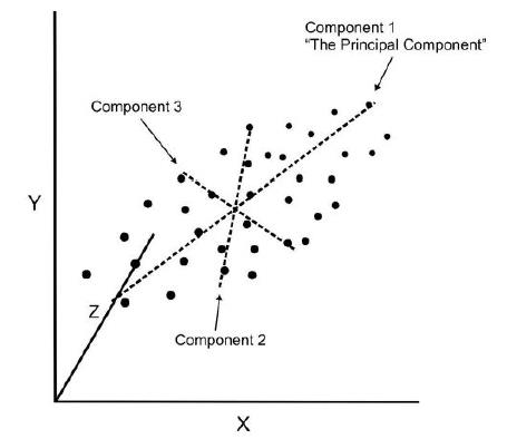
2. Explain Principal Component Analysis?

When we have a large dataset of correlated input variables and we want to reduce the number of input variables to a smaller feature space. while doing this we still want to maintain the critical information. We can solve this by using Principal Component Analysis-PCA.

Now let’s understand the PCA features in little bit more details.

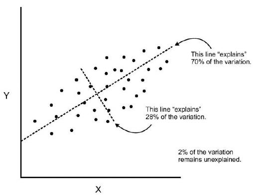
PCA reduce dimensionality of the data using feature extraction. It does this by using variables that help explain most variability of the data in the dataset.

PCA removes redundant information by removing correlated features. PCA creates new independent variables that are independent from each other. This takes care of multicollinearity issue.

PCA is an unsupervised technique. It only looks at the input features and does not take into account the output or the target variable.

3. Importance and limitation of Principal Component Analysis?

Following are the advantages of PCA

• Removes Correlated Features – To visualize our all features in data, we must reduce the same in data, to do that we need to find out the correlation among the features (correlated variables). Finding correlation manually in thousands of features is nearly impossible, frustrating and time-consuming. PCA does this for you efficiently.
• Improve algorithm performance – With so many features, the performance of your algorithm will drastically degrade. PCA is a very common way to speed up your Machine Learning algorithm by getting rid of correlated variables which don’t contribute in any decision making.
• Improve Visualization – It is very hard to visualize and understand the data in high dimensions. PCA transforms a high dimensional data to low dimensional data (2 dimension) so that it can be visualized easily. 

Following are the limitation of PCA

• Independent variable become less interpretable – After implementing PCA on the dataset, your original features will turn into Principal Components. Principal Components are the linear combination of your original features. Principal Components are not as readable and interpretable as original features.
• Data standardization is must before PCA – You must standardize your data before implementing PCA, otherwise PCA will not be able to find the optimal Principal Components.
• Information loss – Although Principal Components try to cover maximum variance among the features in a dataset, if we don’t select the number of Principal Components with care, it may miss some information as compared to the original list of features.

4. What is t-SNE and How to apply t-SNE ?

t-Distributed Stochastic Neighbor Embedding (t-SNE) is an unsupervised, non-linear technique primarily used for data exploration and visualizing high-dimensional data. In simpler terms, t-SNE gives you a feel or intuition of how the data is arranged in a high-dimensional space.

Let’s understand each and every term in details.

Scholastic – Not definite but random probability
Neighbourhood – Concerned only about retaining the structure of neighbourhood points.
Embedding – It means picking up a point from high dimensional space and placing it into lower dimension

5. How to apply t-SNE ?

Basically, it measure similarities between points in the high dimensional space.

Let’s see below image and try to understand the algorithm.

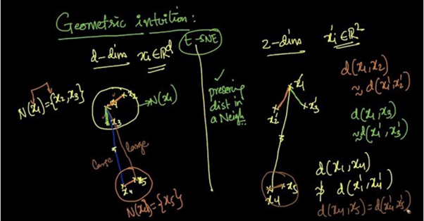
Suppose we are reducing d-dimensional data into 2-dimensional data using t-SNE.
From the above picture we can see that x2 and x3 are in the neighborhood of x1 [N(x1) = {x2, x3}] and x5 is in the neighborhood of x4 [N(x4) = {x5}].

As t-SNE preserves the distances in a neighborhood,

d(x1, x2) ≈ d(x’1, x’2)
d(x1, x3) ≈ d(x’1, x’3)
d(x4, x5) ≈ d(x’4, x’5)

For every point, it constructs a notion of which other points are its ‘neighbors,’ trying to make all points have the same number of neighbors. Then it tries to embed them so that those points all have the same number of neighbors.

6. What is Crowding problem?

Sometimes it is impossible to preserve the distances in all the neighbourhoods. This problem is called Crowding Problem or When we model a high-dimensional dataset in 2 (or 3) dimensions, it is difficult to segregate the nearby datapoints from moderately distant datapoints and gaps can not form between natural clusters.

For example, when a data point, ‘x’ is a neighbor to 2 data points that are not neighboring to each other, this may result in losing the neighborhood of ‘x’ with one of the data points as t-SNE is concerned only within the neighborhood zone.

7. How to interpret t-SNE output?

There are 3 parameters
a) Steps: number of iterations.
b) Perplexity: can be thought of as the number of neighboring points.
c) Epsilon: It is for data visualization and determines the speed which it should be changed.

In real world scenario data analysis tasks involve complex data analysis i.e. analysis for multi-dimensional data. We analyse the data and try to find out various patterns in it.

Here dimensions represents your data point x, As the dimensions of data increases, the difficulty to visualize it and perform computations on it also increases. So, how to reduce the dimensions of a data

• Remove the redundant dimension
• Only keep the most important dimension

To reduce dimensions of the data we use principle component analysis. Before we deep dive in working of PCA, lets understand some key terminology, which will use further.

Variance:

It is a measure of the variability or it simply measures how spread the data set is. Mathematically, it is the average squared deviation from the mean score. We use the following formula to compute variance var(x).

Covariance: It is a measure of the extent to which corresponding elements from two sets of ordered data move in the same direction. Formula is shown above denoted by cov(x,y) as the covariance of x and y.

Here, xi is the value of x in ith dimension. x bar and y bar denote the corresponding mean values.
One way to observe the covariance is how interrelated two data sets are.

Positive, negative and zero covariance:

Positive covariance means X and Y are positively related i.e. as X increases Y also increases. Negative covariance depicts the exact opposite relation. However zero covariance means X and Y are not related.

Eigenvectors and Eigenvalues:

To better understand these concepts, let’s consider the following situation. We are provided with 2-dimensional vectors v1, v2, …, vn. Then, if we apply a linear transformation T (a 2×2 matrix) to our vectors, we will obtain new vectors, called b1, b2,…,bn.

Some of them (more specifically, as many as the number of features), though, have a very interesting property: indeed, once applied the transformation T, they change length but not direction. Those vectors are called eigenvectors, and the scalar which represents the multiple of the eigenvector is called eigenvalue

Thus, each eigenvector has a correspondent eigenvalue.

When should I use PCA:

1. If you want to reduce the number of variables, but aren’t able to identify variables to completely remove from consideration?
2. If you want to ensure your variables are independent from each other.
3. To avoid overfitting your model.
4. If you are comfortable making your independent variable less interpretable.

Background:

• PCA is an unsupervised statistical technique used to examine the interrelations among a set of variables in order to identify the underlying structure of those variables.
• It is also known sometimes as a general factor analysis.
• Where regression determines a line of best fit to a data set, factor analysis determines several orthogonal lines of best fit to the data set.
• Orthogonal means “at right angles”.
  • Actually the lines are perpendicular to each other in n-dimensional space.
• N-dimensional Space is the variable sample space.
  • There are as many dimensions as there are variables, so in a data set with 4 variables the sample space is 4-dimensional.
• Here we have some data plotted along two features, x and y.

• We can add an orthogonal line. Now we can begin to understand the components!

• Components are a linear transformation that chooses a variable system for the data set such that the greatest variance of the data set comes to lie on the first axis.
• The second greatest variance on the second axis, and so on.
• This process allows us to reduce the number of variables used in an analysis.

• We can continue this analysis into higher dimensions.

• If we use this technique on a data set with a large number of variables, we can compress the amount of explained variation to just a few components.
• The most challenging part of PCA is interpreting the components.

For our work with Python, we’ll walk through an example of how to perform PCA with scikit learn. We usually want to standardize our data by some scale for PCA, so we’ll cover how to do this as well.

PCA Algorithm

• Calculate the covariance matrix X of data points.
• Calculate eigenvectors and corresponding eigenvalues.
• Sort the eigen vectors according to their eigenvalues in decreasing order.
• Choose first k eigenvectors and that will be the new k dimensions.
• Transform the original n dimensional data points into k dimensions.

Advantages of PCA

1. Removes Correlated Features: In a real world scenario, this is very common that you get thousands of features in your dataset. You cannot run your algorithm on all the features as it will reduce the performance of your algorithm and it will not be easy to visualize that many features in any kind of graph. So, you MUST reduce the number of features in your dataset. You need to find out the correlation among the features (correlated variables). Finding correlation manually in thousands of features is nearly impossible, frustrating and time-consuming. PCA does this for you efficiently.
2. Improves Algorithm Performance: With so many features, the performance of your algorithm will drastically degrade. PCA is a very common way to speed up your Machine Learning algorithm by getting rid of correlated variables which don’t contribute in any decision making. The training time of the algorithms reduces significantly with less number of features. So, if the input dimensions are too high, then using PCA to speed up the algorithm is a reasonable choice.
3. Improves Visualization: It is very hard to visualize and understand the data in high dimensions. PCA transforms a high dimensional data to low dimensional data (2 dimension) so that it can be visualized easily. We can use 2D Scree Plot to see which Principal Components result in high variance and have more impact as compared to other Principal Components.

Disadvantages of PCA

1. Independent variables become less interpretable: After implementing PCA on the dataset, your original features will turn into Principal Components. Principal Components are the linear combination of your original features. Principal Components are not as readable and interpretable as original features.
2. Data standardization is must before PCA: You must standardize your data before implementing PCA, otherwise PCA will not be able to find the optimal Principal Components. For instance, if a feature set has data expressed in units of Kilograms, Light years, or Millions, the variance scale is huge in the training set. If PCA is applied on such a feature set, the resultant loadings for features with high variance will also be large. Hence, principal components will be biased towards features with high variance, leading to false results.
3. Information Loss: Although Principal Components try to cover maximum variance among the features in a dataset, if we don’t select the number of Principal Components with care, it may miss some information as compared to the original list of features.

Reference:

Medium