Archive March 2020

Principal component Analysis(PCA)-Theory

In real world scenario data analysis tasks involve complex data analysis i.e. analysis for multi-dimensional data. We analyse the data and try to find out various patterns in it.

Here dimensions represents your data point x, As the dimensions of data increases, the difficulty to visualize it and perform computations on it also increases. So, how to reduce the dimensions of a data

  • Remove the redundant dimension
  • Only keep the most important dimension

To reduce dimensions of the data we use principle component analysis. Before we deep dive in working of PCA, lets understand some key terminology, which will use further.

Variance:

It is a measure of the variability or it simply measures how spread the data set is. Mathematically, it is the average squared deviation from the mean score. We use the following formula to compute variance var(x).

Covariance: It is a measure of the extent to which corresponding elements from two sets of ordered data move in the same direction. Formula is shown above denoted by cov(x,y) as the covariance of x and y.

Here, xi is the value of x in ith dimension. x bar and y bar denote the corresponding mean values.
One way to observe the covariance is how interrelated two data sets are.

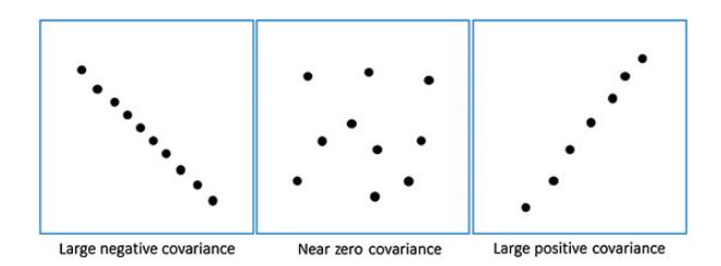
Positive, negative and zero covariance:

Positive covariance means X and Y are positively related i.e. as X increases Y also increases. Negative covariance depicts the exact opposite relation. However zero covariance means X and Y are not related.

Eigenvectors and Eigenvalues:

To better understand these concepts, let’s consider the following situation. We are provided with 2-dimensional vectors v1, v2, …, vn. Then, if we apply a linear transformation T (a 2×2 matrix) to our vectors, we will obtain new vectors, called b1, b2,…,bn.

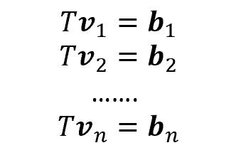
Some of them (more specifically, as many as the number of features), though, have a very interesting property: indeed, once applied the transformation T, they change length but not direction. Those vectors are called eigenvectors, and the scalar which represents the multiple of the eigenvector is called eigenvalue

Thus, each eigenvector has a correspondent eigenvalue.

When should I use PCA:

  1. If you want to reduce the number of variables, but aren’t able to identify variables to completely remove from consideration?
  2. If you want to ensure your variables are independent from each other.
  3. To avoid overfitting your model.
  4. If you are comfortable making your independent variable less interpretable.

Background:

  • PCA is an unsupervised statistical technique used to examine the interrelations among a set of variables in order to identify the underlying structure of those variables.
  • It is also known sometimes as a general factor analysis.
  • Where regression determines a line of best fit to a data set, factor analysis determines several orthogonal lines of best fit to the data set.
  • Orthogonal means “at right angles”.
    • Actually the lines are perpendicular to each other in n-dimensional space.
  • N-dimensional Space is the variable sample space.
    • There are as many dimensions as there are variables, so in a data set with 4 variables the sample space is 4-dimensional.
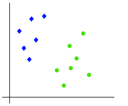
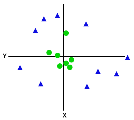
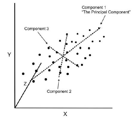
  • Here we have some data plotted along two features, x and y.
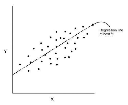
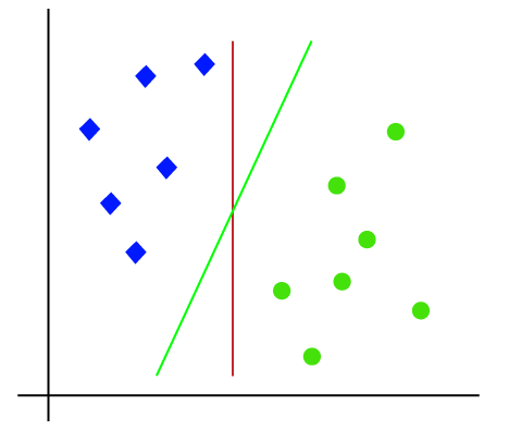
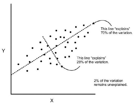
  • We can add an orthogonal line. Now we can begin to understand the components!
  • Components are a linear transformation that chooses a variable system for the data set such that the greatest variance of the data set comes to lie on the first axis.
  • The second greatest variance on the second axis, and so on.
  • This process allows us to reduce the number of variables used in an analysis.
  • We can continue this analysis into higher dimensions.
  • If we use this technique on a data set with a large number of variables, we can compress the amount of explained variation to just a few components.
  • The most challenging part of PCA is interpreting the components.

For our work with Python, we’ll walk through an example of how to perform PCA with scikit learn. We usually want to standardize our data by some scale for PCA, so we’ll cover how to do this as well.

PCA Algorithm

  • Calculate the covariance matrix X of data points.
  • Calculate eigenvectors and corresponding eigenvalues.
  • Sort the eigen vectors according to their eigenvalues in decreasing order.
  • Choose first k eigenvectors and that will be the new k dimensions.
  • Transform the original n dimensional data points into k dimensions.

Advantages of PCA

  1. Removes Correlated Features: In a real world scenario, this is very common that you get thousands of features in your dataset. You cannot run your algorithm on all the features as it will reduce the performance of your algorithm and it will not be easy to visualize that many features in any kind of graph. So, you MUST reduce the number of features in your dataset. You need to find out the correlation among the features (correlated variables). Finding correlation manually in thousands of features is nearly impossible, frustrating and time-consuming. PCA does this for you efficiently.
  2. Improves Algorithm Performance: With so many features, the performance of your algorithm will drastically degrade. PCA is a very common way to speed up your Machine Learning algorithm by getting rid of correlated variables which don’t contribute in any decision making. The training time of the algorithms reduces significantly with less number of features. So, if the input dimensions are too high, then using PCA to speed up the algorithm is a reasonable choice.
  3. Improves Visualization: It is very hard to visualize and understand the data in high dimensions. PCA transforms a high dimensional data to low dimensional data (2 dimension) so that it can be visualized easily. We can use 2D Scree Plot to see which Principal Components result in high variance and have more impact as compared to other Principal Components.

Disadvantages of PCA

  1. Independent variables become less interpretable: After implementing PCA on the dataset, your original features will turn into Principal Components. Principal Components are the linear combination of your original features. Principal Components are not as readable and interpretable as original features.
  2. Data standardization is must before PCA: You must standardize your data before implementing PCA, otherwise PCA will not be able to find the optimal Principal Components. For instance, if a feature set has data expressed in units of Kilograms, Light years, or Millions, the variance scale is huge in the training set. If PCA is applied on such a feature set, the resultant loadings for features with high variance will also be large. Hence, principal components will be biased towards features with high variance, leading to false results.
  3. Information Loss: Although Principal Components try to cover maximum variance among the features in a dataset, if we don’t select the number of Principal Components with care, it may miss some information as compared to the original list of features.

Reference:

Medium

Clustering-Theory

What is Clustering?

Clustering is a most popular unsupervised learning where population or data is grouped based on the similarity of the data-points.

Let’s understand this with an example. Suppose, you are the head of a general store and you want to understand preferences of your costumers to scale up your business. It will not possible for you to look at details of each costumer and devise a unique business strategy for each one of them. But, what you can do is to cluster all of your costumers into say 10 groups based on their purchasing habits and use a separate strategy for costumers in each of these 10 groups. This is called clustering.

To know more about unsupervised learning click here.

Following are the type of clustering application

  • Marketing: Finding groups of customers with similar behaviour given a large database of customer data containing their properties and past buying records.
  • Biology: Classification of plants and animals given their features.
  • Libraries: Book ordering.
  • Insurance: Identifying groups of motor insurance of policy holders with a high average claim cost; identifying frauds.
  • City-planning: Identifying groups of houses according to their house type, value and geographical location
  • Earthquake studies: Clustering helps to observe earthquake epicentres and identify dangerous zones.
  • WWW: Document classification; clustering weblog data to discover groups of similar access patterns

Now let’s discuss the most popular clustering algorithms in detail – K Means clustering and Hierarchical clustering. Let’s begin.

Types of clustering algorithm:

There are several algorithms are available to solve clustering related problem. Every methodology follows a different set of rules for defining the ‘similarity’ among data points. In fact, there are more than 100 clustering algorithms known. But few of the algorithms are very popular, let’s look at them in detail:

Centroid models: This is basically one of iterative clustering algorithm in which the clusters are formed by the closeness of data points to the centroid of clusters. Here, the cluster center i.e. centroid is formed such that the distance of data points is minimum with the center. K-Means clustering algorithm is a popular algorithm that falls into this category. The biggest problem with this algorithm is that we need to specify K in advance.

Distribution models: These clustering models are based on the notion of how probable is it that all data points in the cluster belong to the same distribution (For example: Normal, Gaussian). As distance from the distributions center increases, the probability that a point belongs to the distribution decreases. These models often suffer from overfitting. The bands show that decrease in probability. When you do not know the type of distribution in your data, you should use a different algorithm.

Density Models: Density-based clustering connects areas of high example density into clusters. These algorithms have difficulty with data of varying densities and high dimensions. Further, by design, these algorithms do not assign outliers to clusters.

K Means Clustering:

K means clustering is an effective, widely used, all-around used clustering algorithm. Before actually running it, we have to define a distance function between data points (for example, Euclidean distance if we want to cluster points in space), and we have to set the number of clusters we want (k)

The algorithm begins by selecting k points as starting centroids (‘centers’ of clusters). We can just select any k random points, or we can use some other approach, but picking random points is a good start.

This algorithm works in these 5 steps:

  1. Specify the desired number of clusters K : Let us choose k=2 for these 5 data points in 2-D space.

2. Randomly assign each data point to a cluster : Let’s assign three points in cluster 1 shown using red color and two points in cluster 2 shown using grey color.

3. Compute cluster centroids : The centroid of data points in the red cluster is shown using red cross and those in grey cluster using grey cross.

4. Re-assign each point to the closest cluster centroid : Note that only the data point at the bottom is assigned to the red cluster even though its closer to the centroid of grey cluster. Thus, we assign that data point into grey cluster.

5. Re-compute cluster centroids : Now, re-computing the centroids for both the clusters.

6. Repeat steps 4 and 5 until no improvements are possible : Similarly, we’ll repeat the 4th and 5th steps until we’ll reach global optima. When there will be no further switching of data points between two clusters for two successive repeats. It will mark the termination of the algorithm if not explicitly mentioned

Hierarchical Clustering

Hierarchical clustering creates a tree of clusters. Hierarchical clustering, not surprisingly, is well suited to hierarchical data, such as taxonomies. This algorithm starts with all the data points assigned to a cluster of their own. Then two nearest clusters are merged into the same cluster. In the end, this algorithm terminates when there is only a single cluster left.

There are two important things that we should know about hierarchical clustering:

  • This algorithm has been implemented above using bottom up approach. It is also possible to follow top-down approach starting with all data points assigned in the same cluster and recursively performing splits till each data point is assigned a separate cluster.
  • The decision of merging two clusters is taken on the basis of closeness of these clusters. There are multiple metrics for deciding the closeness of two clusters :
    • Euclidean distance: ||a-b||2 = √(Σ(ai-bi))
    • Squared Euclidean distance: ||a-b||22 = Σ((ai-bi)2)
    • Manhattan distance: ||a-b||1 = Σ|ai-bi|
    • Maximum distance:||a-b||INFINITY = maxi|ai-bi|
    • Mahalanobis distance: √((a-b)T S-1 (-b))   {where, s : covariance matrix}

Difference between K Means and Hierarchical clustering

  • Hierarchical clustering can’t handle big data well but K Means clustering can. This is because the time complexity of K Means is linear i.e. O(n) while that of hierarchical clustering is quadratic i.e. O(n2).
  • In K Means clustering, since we start with random choice of clusters, the results produced by running the algorithm multiple times might differ. While results are reproducible in Hierarchical clustering.
  • K Means is found to work well when the shape of the clusters is hyper spherical (like circle in 2D, sphere in 3D).
  • K Means clustering requires prior knowledge of K i.e. no. of clusters you want to divide your data into. But, you can stop at whatever number of clusters you find appropriate in hierarchical clustering by interpreting the dendrogram

Reference –

AnalyticsVidya

Google Developers

K-Nearest Neighbors (KNN) – Theory

K-nearest neighbors (KNN) algorithm is a type of supervised ML algorithm which can be used for both classification as well as regression problems. However, it is mainly used for classification problems in the industry.

Following are the some important points regarding KNN-algorithm.

  • K-Nearest Neighbor is one of the simplest Machine Learning algorithms based on Supervised Learning technique.
  • K-NN algorithm assumes the similarity between the new case/data and available cases and put the new case into the category that is most similar to the available categories.
  • K-NN algorithm stores all the available data and classifies a new data point based on the similarity. This means when new data appears then it can be easily classified into a well suite category by using K- NN algorithm.
  • K-NN is a non-parametric algorithm, which means it does not make any assumption on underlying data.
  • It is also called a lazy learner algorithm because it does not learn from the training set immediately instead it stores the dataset and at the time of classification, it performs an action on the dataset.
  • KNN algorithm at the training phase just stores the dataset and when it gets new data, then it classifies that data into a category that is much similar to the new data.

Now let’s understand the algorithm with an example.

Suppose, we have an image of a creature that looks similar to cat and dog, but we want to know either it is a cat or dog. So for this identification, we can use the KNN algorithm, as it works on a similarity measure. Our KNN model will find the similar features of the new data set to the cats and dogs images and based on the most similar features it will put it in either cat or dog category.

Why do we need KNN algorithm?

Suppose there are two categories, i.e., Category A and Category B, and we have a new data point x1, so this data point will lie in which of these categories. To solve this type of problem, we need a K-NN algorithm. With the help of K-NN, we can easily identify the category or class of a particular dataset. Consider the below diagram:

How does K-NN work?

To implement KNN algorithm you need to follow following steps.

  • Step-1: Select the number K of the neighbors
  • Step-2: Calculate the Euclidean distance of K number of neighbors
  • Step-3: Take the K nearest neighbors as per the calculated Euclidean distance.
  • Step-4: Among these k neighbors, count the number of the data points in each category.
  • Step-5: Assign the new data points to that category for which the number of the neighbor is maximum.
  • Step-6: Our model is ready.

Suppose we have a new data point and we need to put it in the required category. Consider the below image:

  • First of all, we will choose the number of neighbors, so we will choose the k=5.
  • Next, we will calculate the Euclidean distance between the data points. The Euclidean distance is the distance between two points, which we have already studied in geometry. It can be calculated as:

By calculating the Euclidean distance we got the nearest neighbors, as three nearest neighbors in category A and two nearest neighbors in category B. Consider the below image:

  • As we can see the 3 nearest neighbors are from category A, hence this new data point must belong to category A.

How to select the value of K in the K-NN Algorithm?

Below are some points to remember while selecting the value of K in the K-NN algorithm:

  • There is no particular way to determine the best value for “K”, so we need to try some values to find the best out of them. The most preferred value for K is 5.
  • A very low value for K such as K=1 or K=2, can be noisy and lead to the effects of outliers in the model.
  • Large values for K are good, but it may find some difficulties.

Pros and Cons of KNN:

Pros-

  • Very Simple
  • Training is trivial
  • Works with any number of classes
  • Easy to add more data
  • It has few parameter such as K and distance matric.

Cons-

  • The computation cost is high because of calculating the distance between the data points for all the training samples.
  • Categorical features don’t work well
  • Not good with the high dimensional data

Reference-

Javapoint

Naïve Bayes Classifier-Theory

What is a classifier?

A classifier is a machine learning model that is used to discriminate different objects based on certain features.

Principle of Naive Bayes Classifier:

  • Naïve Bayes algorithm is a supervised learning algorithm, which is based on Bayes theorem and used for solving classification problems.
  • It is mainly used in text classification that includes a high-dimensional training dataset.
  • Naïve Bayes Classifier is one of the simple and most effective Classification algorithms which helps in building the fast machine learning models that can make quick predictions.
  • It is a probabilistic classifier, which means it predicts on the basis of the probability of an object.
  • Some popular examples of Naïve Bayes Algorithm are spam filtration, Sentimental analysis, and classifying articles.

Why is it called Naïve Bayes?

The Naïve Bayes algorithm is comprised of two words Naïve and Bayes, Which can be described as:

  • Naïve: It is called Naïve because it assumes that the occurrence of a certain feature is independent of the occurrence of other features. Such as if the fruit is identified on the bases of color, shape, and taste, then red, spherical, and sweet fruit is recognized as an apple. Hence each feature individually contributes to identify that it is an apple without depending on each other.
  • Bayes: It is called Bayes because it depends on the principle of Bayes Theorem.

Bayes Theorem:

  • Bayes’ theorem is also known as Bayes’ Rule or Bayes’ law, which is used to determine the probability of a hypothesis with prior knowledge. It depends on the conditional probability.
  • The formula for Bayes’ theorem is given as:

Where,

P(A|B) is Posterior probability: Probability of hypothesis A on the observed event B.

P(B|A) is Likelihood probability: Probability of the evidence given that the probability of a hypothesis is true.

P(A) is Prior Probability: Probability of hypothesis before observing the evidence.P(B) is Marginal Probability: Probability of Evidence.

Working of Naïve Bayes Classifier:

Working of Naïve Bayes’ Classifier can be understood with the help of the below example:

Suppose we have a dataset of weather conditions and corresponding target variable “Play“. So using this dataset we need to decide that whether we should play or not on a particular day according to the weather conditions. So to solve this problem, we need to follow the below steps:

  1. Convert the given dataset into frequency tables.
  2. Generate Likelihood table by finding the probabilities of given features.
  3. Now use Bayes theorem to calculate the posterior probability.

Problem: If the weather is sunny, then the Player should play or not?

Solution: To solve this, first consider the below dataset:

Outlook   Play
0 Rainy Yes
1 Sunny Yes
2 Overcast Yes
3 Overcast No
4 Sunny Yes
5 Rainy Yes
6 Sunny Yes
7 Overcast No
8 Rainy No
9 Sunny Yes
10 Sunny No
11 Rainy Yes
12 Overcast Yes
13 Overcast  

Frequency table for the Weather Conditions:

Weather Yes No
Overcast 5 0
Rainy 2 2
Sunny 3 2
Total 10 5

Likelihood table weather condition:

Weather No Yes
Overcast 0 5 5/14= 0.35
Rainy 2 2 4/14=0.29
Sunny 2 3 5/14=0.35
All 4/14=0.29 10/14=0.71

Applying Bayes theorem:

P(Yes|Sunny)= P(Sunny|Yes)*P(Yes)/P(Sunny)

P(Sunny|Yes)= 3/10= 0.3

P(Sunny)= 0.35

P(Yes)=0.71

So P(Yes|Sunny) = 0.3*0.71/0.35= 0.60

P(No|Sunny)= P(Sunny|No)*P(No)/P(Sunny)

P(Sunny|NO)= 2/4=0.5

P(No)= 0.29

P(Sunny)= 0.35

So P(No|Sunny)= 0.5*0.29/0.35 = 0.41

So as we can see from the above calculation that P(Yes|Sunny)>P(No|Sunny)

Hence on a Sunny day, Player can play the game.

Advantages of Naïve Bayes Classifier:

  • Naïve Bayes is one of the fast and easy ML algorithms to predict a class of datasets.
  • It can be used for Binary as well as Multi-class Classifications.
  • It performs well in Multi-class predictions as compared to the other Algorithms.
  • It is the most popular choice for text classification problems.

Disadvantages of Naïve Bayes Classifier:

  • Naive Bayes assumes that all features are independent or unrelated, so it cannot learn the relationship between features.

Applications of Naïve Bayes Classifier:

  • It is used for Credit Scoring.
  • It is used in medical data classification.
  • It can be used in real-time predictions because Naïve Bayes Classifier is an eager learner.
  • It is used in Text classification such as Spam filtering and Sentiment analysis.

Types of Naïve Bayes Model:

There are three types of Naive Bayes Model, which are given below:

  • Gaussian: When the predictors take up a continuous value and are not discrete, we assume that these values are sampled from a gaussian distribution.
  • Multinomial: The Multinomial Naïve Bayes classifier is used when the data is multinomial distributed. It is primarily used for document classification problems, it means a particular document belongs to which category such as Sports, Politics, education, etc.The classifier uses the frequency of words for the predictors.
  • Bernoulli: The Bernoulli classifier works similar to the Multinomial classifier, but the predictor variables are the independent Booleans variables. Such as if a particular word is present or not in a document. This model is also famous for document classification tasks.

Reference:-

Javapoint

Support Vector machine-Theory

Support Vector Machine or SVM is one of the most popular Supervised Learning algorithms, which is used for Classification as well as Regression problems. However, primarily, it is used for Classification problems in Machine Learning.

The goal of the SVM algorithm is to create the best line or decision boundary that can segregate n-dimensional space into classes so that we can easily put the new data point in the correct category in the future. This best decision boundary is called a hyperplane.

SVM chooses the extreme points/vectors that help in creating the hyperplane. These extreme cases are called as support vectors, and hence algorithm is termed as Support Vector Machine. Consider the below diagram in which there are two different categories that are classified using a decision boundary or hyperplane:

Let’s understand SVM through an example.

Suppose we see a strange cat that also has some features of dogs, so if we want a model that can accurately identify whether it is a cat or dog, so such a model can be created by using the SVM algorithm. We will first train our model with lots of images of cats and dogs so that it can learn about different features of cats and dogs, and then we test it with this strange creature. So as support vector creates a decision boundary between these two data (cat and dog) and choose extreme cases (support vectors), it will see the extreme case of cat and dog. On the basis of the support vectors, it will classify it as a cat. Consider the below diagram:

SVM algorithm can be used for Face detection, image classification, text categorization, etc.

Types of SVM:

SVM can be of two types:

  • Linear SVM: Linear SVM is used for linearly separable data, which means if a dataset can be classified into two classes by using a single straight line, then such data is termed as linearly separable data, and classifier is used called as Linear SVM classifier.
  • Non-linear SVM: Non-Linear SVM is used for non-linearly separated data, which means if a dataset cannot be classified by using a straight line, then such data is termed as non-linear data and classifier used is called as Non-linear SVM classifier.

Hyperplane and Support Vectors in the SVM algorithm:

Hyperplane: There can be multiple lines/decision boundaries to segregate the classes in n-dimensional space, but we need to find out the best decision boundary that helps to classify the data points. This best boundary is known as the hyperplane of SVM.

The dimensions of the hyperplane depend on the features present in the dataset, which means if there are 2 features (as shown in image), then hyperplane will be a straight line. And if there are 3 features, then hyperplane will be a 2-dimension plane.

We always create a hyperplane that has a maximum margin, which means the maximum distance between the data points.

How does SVM works?

Linear SVM:

The working of the SVM algorithm can be understood by using an example. Suppose we have a dataset that has two tags (green and blue), and the dataset has two features x1 and x2. We want a classifier that can classify the pair(x1, x2) of coordinates in either green or blue. Consider the below image:

So as it is 2-d space so by just using a straight line, we can easily separate these two classes. But there can be multiple lines that can separate these classes. Consider the below image:

Hence, the SVM algorithm helps to find the best line or decision boundary; this best boundary or region is called as a hyperplane. SVM algorithm finds the closest point of the lines from both the classes. These points are called support vectors. The distance between the vectors and the hyperplane is called as margin. And the goal of SVM is to maximize this margin. The hyperplane with maximum margin is called the optimal hyperplane.

Non-Linear SVM:

If data is linearly arranged, then we can separate it by using a straight line, but for non-linear data, we cannot draw a single straight line. Consider the below image:

So to separate these data points, we need to add one more dimension. For linear data, we have used two dimensions x and y, so for non-linear data, we will add a third dimension z. It can be calculated as:

z=x2 +y2

By adding the third dimension, the sample space will become as below image:

So now, SVM will divide the datasets into classes in the following way. Consider the below image:

Since we are in 3-d Space, hence it is looking like a plane parallel to the x-axis. If we convert it in 2d space with z=1, then it will become as:

Hence we get a circumference of radius 1 in case of non-linear data.

We will see Python Implementation of Support Vector Machine in next chapter

Reference-

Javapoint