Archive 2020

1. What is dimensionality reduction?

When we have a dataset with multiple input features, we know the model will overfit. To reduce input feature space, we can either drop or extract features, this is basically a dimension reduction.

Now let’s discuss more about both techniques.

• Drop irrelevant, redundant features as they do not contribute to the accuracy of the predictive problem. When we drop such input variable, we lose information stored in these variables.
• We can create a new independent variable from existing input variables. This way we do not lose the information in the variables. This is feature extraction

2. Explain Principal Component Analysis?

When we have a large dataset of correlated input variables and we want to reduce the number of input variables to a smaller feature space. while doing this we still want to maintain the critical information. We can solve this by using Principal Component Analysis-PCA.

Now let’s understand the PCA features in little bit more details.

PCA reduce dimensionality of the data using feature extraction. It does this by using variables that help explain most variability of the data in the dataset.

PCA removes redundant information by removing correlated features. PCA creates new independent variables that are independent from each other. This takes care of multicollinearity issue.

PCA is an unsupervised technique. It only looks at the input features and does not take into account the output or the target variable.

3. Importance and limitation of Principal Component Analysis?

Following are the advantages of PCA

• Removes Correlated Features – To visualize our all features in data, we must reduce the same in data, to do that we need to find out the correlation among the features (correlated variables). Finding correlation manually in thousands of features is nearly impossible, frustrating and time-consuming. PCA does this for you efficiently.
• Improve algorithm performance – With so many features, the performance of your algorithm will drastically degrade. PCA is a very common way to speed up your Machine Learning algorithm by getting rid of correlated variables which don’t contribute in any decision making.
• Improve Visualization – It is very hard to visualize and understand the data in high dimensions. PCA transforms a high dimensional data to low dimensional data (2 dimension) so that it can be visualized easily. 

Following are the limitation of PCA

• Independent variable become less interpretable – After implementing PCA on the dataset, your original features will turn into Principal Components. Principal Components are the linear combination of your original features. Principal Components are not as readable and interpretable as original features.
• Data standardization is must before PCA – You must standardize your data before implementing PCA, otherwise PCA will not be able to find the optimal Principal Components.
• Information loss – Although Principal Components try to cover maximum variance among the features in a dataset, if we don’t select the number of Principal Components with care, it may miss some information as compared to the original list of features.

4. What is t-SNE and How to apply t-SNE ?

t-Distributed Stochastic Neighbor Embedding (t-SNE) is an unsupervised, non-linear technique primarily used for data exploration and visualizing high-dimensional data. In simpler terms, t-SNE gives you a feel or intuition of how the data is arranged in a high-dimensional space.

Let’s understand each and every term in details.

Scholastic – Not definite but random probability
Neighbourhood – Concerned only about retaining the structure of neighbourhood points.
Embedding – It means picking up a point from high dimensional space and placing it into lower dimension

5. How to apply t-SNE ?

Basically, it measure similarities between points in the high dimensional space.

Let’s see below image and try to understand the algorithm.

Suppose we are reducing d-dimensional data into 2-dimensional data using t-SNE.
From the above picture we can see that x2 and x3 are in the neighborhood of x1 [N(x1) = {x2, x3}] and x5 is in the neighborhood of x4 [N(x4) = {x5}].

As t-SNE preserves the distances in a neighborhood,

d(x1, x2) ≈ d(x’1, x’2)
d(x1, x3) ≈ d(x’1, x’3)
d(x4, x5) ≈ d(x’4, x’5)

For every point, it constructs a notion of which other points are its ‘neighbors,’ trying to make all points have the same number of neighbors. Then it tries to embed them so that those points all have the same number of neighbors.

6. What is Crowding problem?

Sometimes it is impossible to preserve the distances in all the neighbourhoods. This problem is called Crowding Problem or When we model a high-dimensional dataset in 2 (or 3) dimensions, it is difficult to segregate the nearby datapoints from moderately distant datapoints and gaps can not form between natural clusters.

For example, when a data point, ‘x’ is a neighbor to 2 data points that are not neighboring to each other, this may result in losing the neighborhood of ‘x’ with one of the data points as t-SNE is concerned only within the neighborhood zone.

7. How to interpret t-SNE output?

There are 3 parameters
a) Steps: number of iterations.
b) Perplexity: can be thought of as the number of neighboring points.
c) Epsilon: It is for data visualization and determines the speed which it should be changed.

How do you assess the statistical significance of an insight?

We need to perform hypothesis testing to determine statistical significance. Will take following steps.

• First will define null hypothesis and alternate hypothesis
• We will calculate p- value
• Last, we would set the level of the significance (alpha) and if the p-value is less than the alpha, you would reject the null — in other words, the result is statistically significant.

What is the Central Limit Theorem and why is it important?

• Central limit theorem is very important concept in stats. It states that no matter the underlying distribution of the data set, the sampling distribution would be equal to the mean of original distribution and variance would be n times smaller, where n is the size of sample
• The central limit theorem (CLT) states that the distribution of sample means approximates a normal distribution as the sample size gets larger.
• Sample sizes equal to or greater than 30 are considered sufficient for the CLT to hold.
• A key aspect of CLT is that the average of the sample means and standard deviations will equal the population mean and standard deviation.

Example-

Suppose that we are interested in estimating the average height among all people. Collecting data for every person in the world is impossible. While we can’t obtain a height measurement from everyone in the population, we can still sample some people. The question now becomes, what can we say about the average height of the entire population given a single sample. The Central Limit Theorem addresses this question exactly.”

What is sampling? How many sampling methods do you know?

Data sampling is a statistical analysis technique used to select, manipulate and analyse a subset of data points to identify patterns and trends in the larger data set. It enables data scientists and other data analysts to work with a small, manageable amount of data about a statistical population to build and run analytical models more quickly, while still producing accurate findings.

• Simple random sampling: Software is used to randomly select subjects from the whole population.
• Stratified sampling: Subsets of the data sets or population are created based on a common factor, and samples are randomly collected from each subgroup.
• Cluster sampling: The larger data set is divided into subsets (clusters) based on a defined factor, then a random sampling of clusters is analyzed.
• Multistage sampling: A more complicated form of cluster sampling, this method also involves dividing the larger population into a number of clusters. Second-stage clusters are then broken out based on a secondary factor, and those clusters are then sampled and analyzed. This staging could continue as multiple subsets are identified, clustered and analyzed.
• Systematic sampling: A sample is created by setting an interval at which to extract data from the larger population — for example, selecting every 10th row in a spreadsheet of 200 items to create a sample size of 20 rows to analyze.

Explain selection bias (with regard to a dataset, not variable selection). Why is it important? How can data management procedures such as missing data handling make it worse?

Selection bias is the phenomenon of selecting individuals, groups or data for analysis in such a way that proper randomization is not achieved, ultimately resulting in a sample that is not representative of the population.

Types of selection bias include:

• sampling bias: a biased sample caused by non-random sampling
• time interval: selecting a specific time frame that supports the desired conclusion. e.g. conducting a sales analysis near Christmas.
• attrition: attrition bias is similar to survivorship bias, where only those that ‘survived’ a long process are included in an analysis, or failure bias, where those that ‘failed’ are only included
• observer selection: related to the Anthropic principle, which is a philosophical consideration that any data we collect about the universe is filtered by the fact that, in order for it to be observable, it must be compatible with the conscious and sapient life that observes it. 

Handling missing data can make selection bias worse because different methods impact the data in different ways. For example, if you replace null values with the mean of the data, you adding bias in the sense that you’re assuming that the data is not as spread out as it might actually be.

What is the difference between type I vs type II error?

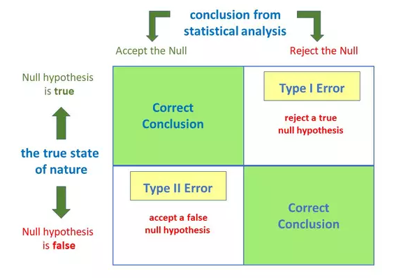
Anytime we make a decision using statistics there are four possible outcomes, with two representing correct decisions and two representing errors.

Type – I Error:

A type 1 error is also known as a false positive and occurs when a researcher incorrectly rejects a true null hypothesis. This means that your report that your findings are significant when in fact they have occurred by chance.

The probability of making a type I error is represented by your alpha level (α), which is the p-value. A p-value of 0.05 indicates that you are willing to accept a 5% chance that you are wrong when you reject the null hypothesis

Type – II Error:

A type II error is also known as a false negative and occurs when a researcher fails to reject a null hypothesis which is really false. Here a researcher concludes there is not a significant effect, when actually there really is.

The probability of making a type II error is called Beta (β), and this is related to the power of the statistical test (power = 1- β). You can decrease your risk of committing a type II error by ensuring your test has enough power.

What are the four main things we should know before studying data analysis?

Following are the key point that we should know:

• Descriptive statistics
• Inferential statistics
• Distributions (normal distribution / sampling distribution)
• Hypothesis testing

What is the difference between inferential statistics and descriptive statistics?

Descriptive Analysis – It uses the data to provide description of the population either through numerical calculations or graph or tables.

Inferential statistics – Provides information of a sample and we need to inferential statistics to reach to a conclusion about the population.

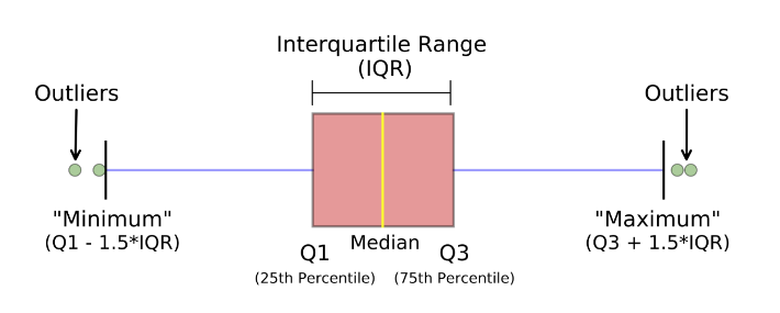
How to calculate range and interquartile range?

IQR = Q3 – Q1

Where, Q3 is the third quartile (75 percentile) 

Where, Q1 is the first quartile (25 percentile)

What is the benefit of using box plot?

A box plot, also known as a box and whisker plot, is a type of graph that displays a summary of a large amount of data in five numbers. These numbers include the median, upper quartile, lower quartile, minimum and maximum data values.

Following are the advantages of Box-plot:

• Handle Large data easily – Due to the five-number data summary, a box plot can handle and present a summary of a large amount of data. Organizing data in a box plot by using five key concepts is an efficient way of dealing with large data too unmanageable for other graphs, such as line plots or stem and leaf plots.
• A box plot shows only a simple summary of the distribution of results, so that it you can quickly view it and compare it with other data.
• A box plot is a highly visually effective way of viewing a clear summary of one or more sets of data. 
• A box plot is one of very few statistical graph methods that show outliers. Any results of data that fall outside of the minimum and maximum values known as outliers are easy to determine on a box plot graph.

What is the meaning of standard deviation?

It represents how far are the data points from the mean

(σ) = √(∑(x-µ)² / n)

Variance is the square of standard deviation

What is left skewed distribution and right skewed distribution?

Left skewed

• The left tail is longer than the right side
  • Mean < median < mode

Right skewed

• The right tail is longer than the left side
  • Mode < median < mean

What does symmetric distribution mean?

The part of the distribution that is on the left side of the median is same as the part of the distribution that is on the right side of the median

Few examples are – uniform distribution, binomial distribution, normal distribution

What is the relationship between mean and median in normal distribution?

In the normal distribution mean is equal to median

What does it mean by bell curve distribution and Gaussian distribution?

Normal distribution is called bell curve distribution / Gaussian distribution.It is called bell curve because it has the shape of a bell.It is called Gaussian distribution as it is named after Carl Gauss.

How to convert normal distribution to standard normal distribution?

Standardized normal distribution has mean = 0 and standard deviation = 1. To convert normal distribution to standard normal distribution we can use the formula

X (standardized) = (x-µ) / σ

What is an outlier? What can I do with outlier?

An outlier is an abnormal value (It is at an abnormal distance from rest of the data points). 

Following thing we can do with outliers

Remove outlier

• When we know the data-point is wrong (negative age of a person)
  • When we have lots of data
  • We should provide two analyses. One with outliers and another without outliers.

Keep outlier

• When there are lot of outliers (skewed data)
  • When results are critical
  • When outliers have meaning (fraud data)

What is the difference between population parameters and sample statistics?

Population parameters are:

• Mean = µ
  • Standard deviation = σ

Sample statistics are:

• Mean = x (bar)
  • Standard deviation = s

How to find the mean length of all fishes in the sea?

Define the confidence level (most common is 95%). Take a sample of fishes from the sea (to get better results the number of fishes > 30). Calculate the mean length and standard deviation of the lengths. Calculate t-statistics. Get the confidence interval in which the mean length of all the fishes should be.

What are the effects of the width of confidence interval?

• Confidence interval is used for decision making
• As the confidence level increases the width of the confidence interval also increases
• As the width of the confidence interval increases, we tend to get useless information also.

Mention the relationship between standard error and margin of error?

As the standard error increases the margin of error also increases.

What is p-value and what does it signify?

The p-value reflects the strength of evidence against the null hypothesis. p-value is defined as the probability that the data would be at least as extreme as those observed, if the null hypothesis were true.

• P- Value > 0.05 denotes weak evidence against the null hypothesis which means the null hypothesis cannot be rejected.
• P-value < 0.05 denotes strong evidence against the null hypothesis which means the null hypothesis can be rejected.
• P-value=0.05 is the marginal value indicating it is possible to go either way.

How to calculate p-value using manual method?

• Find H0 and H1
• Find n, x(bar) and s
• Find DF for t-distribution
• Find the type of distribution – t or z distribution
• Find t or z value (using the look-up table)
• Compute the p-value to critical value

What is the difference between one tail and two tail hypothesis testing?

• Two tail test – When null hypothesis contain an equality (=) or inequality sign (<>)
• One tail test – When the null hypothesis does not contain equality (=) or inequality sign (<, >, <=, >= )

What is A/B testing?

A/B testing is a form of hypothesis testing and two-sample hypothesis testing to compare two versions, the control and variant, of a single variable. It is commonly used to improve and optimize user experience and marketing.

What is R-squared and Adjusted R-square?

R-squared or R2 is a  value in which your input variables explain the variation of your output / predicted variable. So, if R-square is 0.8, it means 80% of the variation in the output variable is explained by the input variables. So, in simple terms, higher the R squared, the more variation is explained by your input variables and hence better is your model.

However, the problem with R-squared is that it will either stay the same or increase with addition of more variables, even if they do not have any relationship with the output variables. This is where “Adjusted R square” comes to help. Adjusted R-square penalizes you for adding variables which do not improve your existing model.

Hence, if you are building Linear regression on multiple variable, it is always suggested that you use Adjusted R-squared to judge goodness of model. In case you only have one input variable, R-square and Adjusted R squared would be exactly same.

Typically, the more non-significant variables you add into the model, the gap in R-squared and Adjusted R-squared increases.

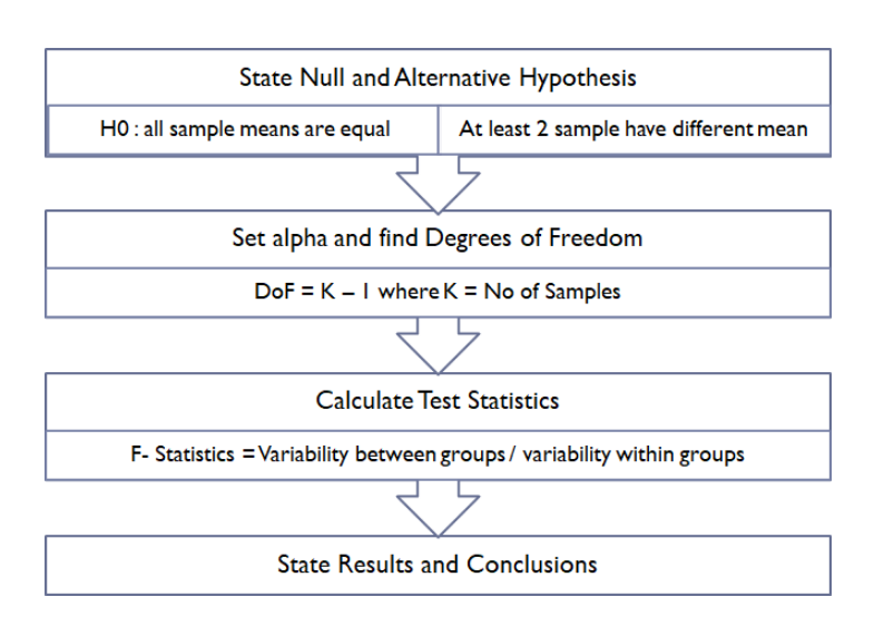
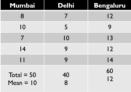
Explain ANOVA and it’s applications?

Analysis of Variance (abbreviated as ANOVA) is an extremely useful technique which is used to compare the means of multiple samples. Whether there is a significant difference between the mean of 2 samples, can be evaluated using z-test or t-test but in case of more than 2 samples, t-test can not be applied as it accumulates the error and it will be cumbersome as the number of sample will increase (for example: for 4 samples — 12 t-test will have to be performed). The ANOVA technique enables us to perform this simultaneous test. Here is the procedure to perform ANOVA.

Let’s see with example: Imagine we want to compare the salary of Data Scientist across 3 cities of india — Bengaluru, Delhi and Mumbai. In order to do so, we collected data shown below.

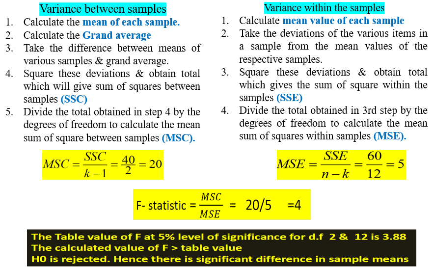
Following picture explains the steps followed to get the Anova results

There is a limitation of ANOVA that it does not tell which pair is having significant difference. In above example, It is clear that there is a significant difference between the means of Data Scientist salary among these 3 cities but it does not provide any information on which pair is having the significant difference

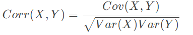
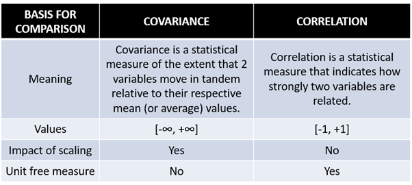
What is the difference between Correlation and Covariance?

Correlation and Covariance are statistical concepts which are generally used to determine the relationship and measure the dependency between two random variables. Actually, Correlation is a special case of covariance which can be observed when the variables are standardized. This point will become clear from the formulas :

Here listed key differences between covariance and correlation

Reference –

Analyticsindiamag

Towardsdatascience

Springboard

Variables are nothing but reserved memory locations to store values. This means that when you create a variable you reserve some space in memory. Variable also known as identifier and used to hold value.

In Python, we don’t need to specify the type of variable, because Python is language and smart enough to get variable type.

How to define Variable Names

A variable can have a short name (like x and y) or a more descriptive name (age, carname, total_volume). Rules for Python variables:

• A variable name must start with a letter or the underscore character
• A variable name cannot start with a number
• A variable name can only contain alpha-numeric characters and underscores (A-z, 0-9, and _ )
• Variable names are case-sensitive (age, Age and AGE are three different variables)

Declaring Variable and Assigning Values

Python allows us to create variable at required time. It does not bound us to declare variable before using in the application. We don’t need to declare explicitly variable in Python. When we assign any value to the variable that variable is declared automatically.

The equal (=) operator is used to assign value to a variable.

counter = 100 # An integer assignment
miles = 1000.0 # A floating point
name = “John” # A string

Here, 100, 1000.0 and “John” are the values assigned to counter, miles, and name variables, respectively.

Multiple Assignments

Python allows us to assign a value to multiple variables in a single statement which is also known as multiple assignments. We can apply multiple assignments in two ways either by assigning a single value to multiple variables or assigning multiple values to multiple variables. Lets see given examples.

X = Y = Z = 50

Let’s explore above concept through jupyter notebook

In this lecture, we will learn about numbers in Python and how to use them.

We’ll learn about the following topics:

1.) Types of Numbers in Python

2.) Basic Arithmetic

3.) Differences between classic division and floor division

4.) Object Assignment in Python

Types of numbers:

There are three numeric types in Python

• int
• float
• complex

Variables of numeric types are created when you assign a value to them:

x = 1    # int
y = 2.8  # float
z = 1j   # complex

Let’s explore about the numbers through jupyter notebook.

String literals in python are surrounded by either single quotation marks, or double quotation marks.

• ‘hello’ is the same as “hello”.
• You can display a string literal with the print() function.

Let’s explore string concept through jupyter notebook.

String formatting lets you inject items into a string rather than trying to chain items together using commas or string concatenation. As a quick comparison, consider:

player = ‘Thomas’
points = 33
‘Last night, ‘+player+’ scored ‘+str(points)+’ points.’ # concatenation
f’Last night, {player} scored {points} points.’ # string formatting

There are three ways to perform string formatting.

• The oldest method involves placeholders using the modulo % character.
• An improved technique uses the .format() string method.
• The newest method, introduced with Python 3.6, uses formatted string literals, called f-strings.

Since you will likely encounter all three versions in someone else’s code, we describe each of them here.

Let’s explore the concept through jupyter notebook.

List is a collection which is ordered and changeable. It allows duplicate members.

A list can be defined as a collection of values or items of different types. The items in the list are separated with the comma (,) and enclosed with the square brackets [].

A list can be defined as follows.

L1 = [“John”, 102, “USA”]
L2 = [1, 2, 3, 4, 5, 6]
L3 = [1, “Ryan”]

Let’s explore more concepts about list through following jupyter notebook exercise.

A dictionary is a collection which is unordered, changeable and indexed. In Python dictionaries are written with curly brackets, and they have keys and values.

Example:
dict = {‘Name’: ‘Zara’, ‘Age’: 7, ‘Class’: ‘First’}
print “dict[‘Name’]: “, dict[‘Name’]
print “dict[‘Age’]: “, dict[‘Age’]

When the above code is executed, it produces the following result

dict[‘Name’]: Zara
dict[‘Age’]: 7

Let’s Explore more about dictionaries through jupyter notebook.

A tuple is a collection which is ordered and unchangeable. In Python tuples are written with round brackets.

Example –

tup1 = (‘physics’, ‘chemistry’, 1997, 2000);
tup2 = (1, 2, 3, 4, 5 );

Let’s explore more about tuple through jupyter notebook.

A set is a collection which is unordered and unindexed. In Python sets are written with curly brackets.

Example:

thisset = {“apple”, “banana”, “cherry”}

Access Items

You cannot access items in a set by referring to an index, since sets are unordered the items has no index.

But you can loop through the set items using a for loop, or ask if a specified value is present in a set, by using the in keyword.

Let’s explore Sets and Booleans concepts with Jupyter notebook.