Archive May 2021

SQL Interview Questions and answers – 2021

1. What is DBMS?

A Database Management System (DBMS) is a program that controls creation, maintenance and use of a database. DBMS can be termed as File Manager that manages data in a database rather than saving it in file systems.

Database Management System (DBMS) is a software application that interacts with the user, applications, and the database itself to capture and analyze data. A database is a structured collection of data. 

A DBMS allows a user to interact with the database. The data stored in the database can be modified, retrieved and deleted and can be of any type like strings, numbers, images, etc.

There are two types of DBMS:

  • Relational Database Management System: The data is stored in relations (tables). Example – MySQL.
  • Non-Relational Database Management System: There is no concept of relations, tuples and attributes.  Example – MongoDB

2. What is RDBMS?

RDBMS stands for Relational Database Management System. RDBMS store the data into the collection of tables, which is related by common fields between the columns of the table. It also provides relational operators to manipulate the data stored into the tables.

3. What is SQL?

SQL stands for the Structured Query Language. SQL is a standard query language used for maintaining the relational database and perform many different operations of data manipulation on the data. SQL initially was invented in 1970. It is a database language used for database creation, deletion, fetching rows and modifying rows, etc. sometimes it is pronounced as ‘sequel.’

4. What are the usages of SQL?

  • SQL is responsible for maintaining the relational data and the data structures present in the database.
  • To execute queries against a database
  • To retrieve data from a database
  • To inserts records in a database
  • To updates records in a database
  • To delete records from a database
  • To create new databases
  • To create new tables in a database
  • To create views in a database
  • To perform complex operations on the database.

5. Does SQL support programming?

SQL refers to the Standard Query Language, which is not actually the programming language. SQL doesn’t have a loop, Conditional statement, logical operations, it can not be used for anything other than data manipulation. It is used like commanding (Query) language to access databases. The primary purpose of SQL is to retrieve, manipulate, update and perform complex operations like joins on the data present in the database.

6. What do you mean by table and field in SQL?

A table refers to a collection of data in an organised manner in form of rows and columns. A field refers to the number of columns in a table.

For example:

Table:StudentInformation
Field: Stu Id, Stu Name, Stu Marks

7. What are joins in SQL?

A JOIN clause is used to combine rows from two or more tables, based on a related column between them. It is used to merge two tables or retrieve data from there. There are 4 types of joins, as you can refer to below:
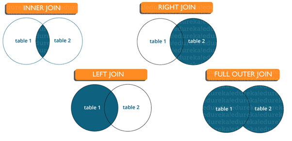
Inner join: Inner Join in SQL is the most common type of join. It is used to return all the rows from multiple tables where the join condition is satisfied. 

Left Join:  Left Join in SQL is used to return all the rows from the left table but only the matching rows from the right table where the join condition is fulfilled.

Right Join: Right Join in SQL is used to return all the rows from the right table but only the matching rows from the left table where the join condition is fulfilled.

Full Join: Full join returns all the records when there is a match in any of the tables. Therefore, it returns all the rows from the left-hand side table and all the rows from the right-hand side table.

8. What is a Database?

Database is nothing but an organized form of data for easy access, storing, retrieval and managing of data. This is also known as structured form of data which can be accessed in many ways.

Example: School Management Database, Bank Management Database.

9. What is a primary key?

A primary key is a combination of fields which uniquely specify a row. This is a special kind of unique key, and it has implicit NOT NULL constraint. It means, Primary key values cannot be NULL.

10. What is a unique key?

A Unique key constraint uniquely identified each record in the database. This provides uniqueness for the column or set of columns.

A Primary key constraint has automatic unique constraint defined on it. But not, in the case of Unique Key.

There can be many unique constraint defined per table, but only one Primary key constraint defined per table.

11. What is a foreign key?

A foreign key is one table which can be related to the primary key of another table. Relationship needs to be created between two tables by referencing foreign key with the primary key of another table.

12. What is a Self-Join?

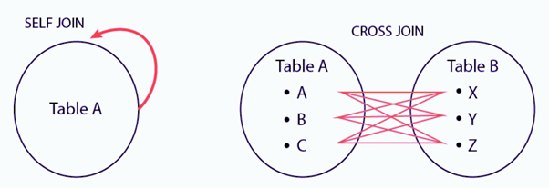
A self JOIN is a case of regular join where a table is joined to itself based on some relation between its own column(s). Self-join uses the INNER JOIN or LEFT JOIN clause and a table alias is used to assign different names to the table within the query.

SELECT A.emp_id AS "Emp_ID",A.emp_name AS "Employee",
B.emp_id AS "Sup_ID",B.emp_name AS "Supervisor"
FROM employee A, employee B
WHERE A.emp_sup = B.emp_id;

13. What is a Cross-Join?

Cross join can be defined as a cartesian product of the two tables included in the join. The table after join contains the same number of rows as in the cross-product of number of rows in the two tables. If a WHERE clause is used in cross join then the query will work like an INNER JOIN.

SELECT stu.name, sub.subject 
FROM students AS stu
CROSS JOIN subjects AS sub;
14. What is the difference between CHAR and VARCHAR2 datatype in SQL?

Both Char and Varchar2 are used for characters datatype but varchar2 is used for character strings of variable length whereas Char is used for strings of fixed length. For example, char(10) can only store 10 characters and will not be able to store a string of any other length whereas varchar2(10) can store any length i.e 6,8,2 in this variable.

15. What are Constraints?

Constraints in SQL are used to specify the limit on the data type of the table. It can be specified while creating or altering the table statement. The sample of constraints are:

  • NOT NULL
  • CHECK
  • DEFAULT
  • UNIQUE
  • PRIMARY KEY
  • FOREIGN KEY

16. What is the difference between DELETE and TRUNCATE statements?

DELETETRUNCATE
Delete command is used to delete a row in a table.Truncate is used to delete all the rows from a table.
You can rollback data after using delete statement.You cannot rollback data.
It is a DML command.It is a DDL command.
It is slower than truncate statement.It is faster.

17. What do you mean by data integrity? 

Data Integrity defines the accuracy as well as the consistency of the data stored in a database. It also defines integrity constraints to enforce business rules on the data when it is entered into an application or a database.

18. What is an Index?

An Index in a relational database is a data structure that improves the speed of data retrieval operations on a table. Indexes allow the database to find and retrieve specific rows much faster than scanning the entire table.

Key Features of an Index:
  • Improves Query Performance: Indexes reduce the time it takes to perform SELECT queries and JOIN operations by allowing the database to quickly locate the data.
  • Created on Columns: Indexes are typically created on one or more columns of a table. These columns are often the ones most frequently searched or used in WHERE clauses.
  • Supports Uniqueness: Some indexes, like the primary key index, enforce the uniqueness of values in a column.
Types of Indexes:

Primary Index:

  • Automatically created when a primary key is defined.
  • Enforces uniqueness and is used to speed up data access.

Unique Index:

  • Ensures that no duplicate values are allowed in the indexed column.
  • Similar to a primary index but can be applied to non-primary key columns.

Clustered Index:

  • Determines the physical order of data in a table. The table itself is organized based on this index.
  • Only one clustered index is allowed per table because the data rows can only be sorted in one way.

Non-Clustered Index:

  • Does not alter the physical order of the data. Instead, it creates a separate structure (like a lookup table) that references the data.
  • A table can have multiple non-clustered indexes.

Composite Index:

  • An index on multiple columns. It is useful when queries involve conditions on more than one column.

Full-Text Index:

  • Used for searching large text-based columns (like documents, descriptions).
  • Supports advanced searching capabilities like searching for keywords, phrases, and proximity searches.

Bitmap Index:

  • Typically used in data warehousing environments.
  • Efficient for columns with low cardinality (few distinct values).
How Indexes Work:

Indexes function like a book’s index, allowing quick lookups by pointing directly to where the data is located. For example, if you have an index on the customer_name column, searching for a specific name doesn’t require scanning the entire table row by row; instead, the index is consulted to find the relevant rows directly.

Drawbacks of Indexes:
  • Storage Overhead: Indexes require additional disk space.
  • Slower Write Operations: Insert, update, and delete operations become slower because indexes need to be updated when the data changes.
  • Maintenance: Indexes require maintenance and tuning to ensure optimal performance as the data grows.
Example of Creating an Index:
CREATE INDEX idx_customer_name ON customers(customer_name);

This creates a non-clustered index on the customer_name column of the customers table.

When to Use Indexes:
  • When a column is frequently used in WHERE clauses.
  • When a column is frequently used in JOIN operations.
  • When you need to enforce uniqueness (unique indexes).
  • For speeding up queries on large tables.

Conclusion:

Indexes are powerful tools to optimize query performance, but they need to be used strategically to balance query speed with write performance and storage considerations.

19. Explain different types of index in SQL.

There are three types of index in SQL namely:

Unique Index:

This index does not allow the field to have duplicate values if the column is unique indexed. If a primary key is defined, a unique index can be applied automatically.

CREATE UNIQUE INDEX myIndex
ON students (enroll_no);

Clustered Index:

This index reorders the physical order of the table and searches based on the basis of key values. Each table can only have one clustered index.

Non-Clustered Index:

Non-Clustered Index does not alter the physical order of the table and maintains a logical order of the data. Each table can have many non clustered indexes.

20. What is a Data Definition Language?

Data definition language (DDL) is the subset of the database which defines the data structure of the database in the initial stage when the database is about to be created. It consists of the following commands: CREATE, ALTER and DELETE database objects such as schema, tables, view, sequence, etc.

21. What is a Data Manipulation Language?

Data manipulation language makes the user able to retrieve and manipulate data. It is used to perform the following operations.

  • Insert data into database through INSERT command.
  • Retrieve data from the database through SELECT command.
  • Update data in the database through UPDATE command.
  • Delete data from the database through DELETE command.

22. What is Data Control Language?

Data control language allows you to control access to the database. DCL is the only subset of the database which decides that what part of the database should be accessed by which user at what point of time. It includes two commands GRANT and REVOKE.

GRANT: to grant the specific user to perform a particular task

REVOKE: to cancel previously denied or granted permissions.

23. What is Normalization in SQL?

Normalization in SQL is a process of organizing the data in a database to reduce redundancy and improve data integrity. The main goal of normalization is to divide large tables into smaller, more manageable ones while defining relationships between them, ensuring that each piece of data is stored in one place only.

Key Objectives of Normalization:

  1. Eliminate Redundant Data: Ensure that no unnecessary duplicate data is stored.
  2. Ensure Data Integrity: Reduce the chances of anomalies like update, insert, and delete anomalies.
  3. Efficient Data Management: Normalize tables to streamline data management and reduce complexity.

Normal Forms:

Normalization is typically carried out in steps, referred to as “normal forms,” with each form addressing specific issues:

  1. First Normal Form (1NF):
  • Ensures that all columns contain atomic (indivisible) values.
  • Each column must have a unique name.
  • All entries in a column must be of the same data type.
  1. Second Normal Form (2NF):
  • Achieves 1NF.
  • Ensures that all non-key attributes are fully dependent on the primary key. This eliminates partial dependencies, where an attribute depends only on part of a composite key.
  1. Third Normal Form (3NF):
  • Achieves 2NF.
  • Removes transitive dependencies, where non-key attributes depend on other non-key attributes.
  1. Boyce-Codd Normal Form (BCNF):
  • A stricter version of 3NF, ensuring that every determinant is a candidate key.
  1. Fourth Normal Form (4NF) and Fifth Normal Form (5NF):
  • These deal with more complex situations involving multi-valued dependencies and join dependencies, respectively.
Example:

Consider a table storing information about students and courses:

StudentIDStudentNameCourseIDCourseName
1Alice101Math
1Alice102Physics
2Bob101Math

Here, student information is repeated if they are enrolled in multiple courses. By normalizing:

  1. Split into separate tables:
  • Students Table: (StudentID, StudentName)
  • Courses Table: (CourseID, CourseName)
  • Enrollments Table: (StudentID, CourseID)

This structure removes redundancy and reduces anomalies.

In summary, normalization is crucial for creating efficient and scalable databases.

24. What is pl sql?

PL SQL stands for Procedural language constructs for Structured Query Language. PL SQL was introduced by Oracle to overcome the limitations of plain sql. So, pl sql adds in procedural language approach to the plain vanilla sql.

While, with the help of sql, we were able to DDL and DML queries, with the help of PL SQL, we will be able to create functions, triggers and other procedural constructs.

25. What is ETL in SQL?

ETL stands for Extract, Transform and Load. It is a three step process, where we would have to start off by extracting the data from sources. Once we collate the data from different sources, what we have is raw data. This raw data has to be transformed into tidy format, which will come in the second phase. Finally, we would have to load this tidy data into tools which would help us to find insights.

26. What is OLAP?

OLAP stands for Online Analytical Processing. And a class of software programs which are characterized by relatively low frequency of online transactions. Queries are often too complex and involve a bunch of aggregations.

27. What is a “TRIGGER” in SQL?

  • A trigger allows you to execute a batch of SQL code when an insert, update or delete command is run against a specific table as TRIGGER is said to be the set of actions that are performed whenever commands like insert, update or delete are given through queries.
  • The trigger is said to be activated when these commands are given to the system.
  • Triggers are the particular type of stored procedures that are defined to execute automatically in place or after data modifications.
  • Triggers are generated using CREATE TRIGGER statement.

28. What is ACID property in a database?

ACID property is used to ensure that the data transactions are processed reliably in a database system.

A single logical operation of a data is called transaction.

ACID is an acronym for Atomicity, Consistency, Isolation, Durability.

Atomicity: it requires that each transaction is all or nothing. It means if one part of the transaction fails, the entire transaction fails and the database state is left unchanged.

Consistency: the consistency property ensure that the data must meet all validation rules. In simple words you can say that your transaction never leaves your database without completing its state.

Isolation: this property ensure that the concurrent property of execution should not be met. The main goal of providing isolation is concurrency control.

Durability: durability simply means that once a transaction has been committed, it will remain so, come what may even power loss, crashes or errors.

29. What are the syntax and use of the COALESCE function?

The syntax of COALESCE function:

COALESCE(exp1, exp2, …. expn) 

The COALESCE function is used to return the first non-null expression given in the parameter list.

30. What is the SQL query to display the current date?

There is a built-in function in SQL called GetDate() which is used to return the current timestamp.

31. Are NULL values same as that of zero or a blank space?

A NULL value is not at all same as that of zero or a blank space. NULL value represents a value which is unavailable, unknown, assigned or not applicable whereas a zero is a number and blank space is a character.

32. What is subquery in SQL?

A subquery is a query inside another query where a query is defined to retrieve data or information back from the database. In a subquery, the outer query is called as the main query whereas the inner query is called subquery. Subqueries are always executed first and the result of the subquery is passed on to the main query. It can be nested inside a SELECT, UPDATE or any other query. A subquery can also use any comparison operators such as >,< or =.

33. What is the difference between ‘HAVING’ CLAUSE and a ‘WHERE’ CLAUSE?

HAVING clause can be used only with SELECT statement. It is usually used in a GROUP BY clause and whenever GROUP BY is not used, HAVING behaves like a WHERE clause.
Having Clause is only used with the GROUP BY function in a query whereas WHERE Clause is applied to each row before they are a part of the GROUP BY function in a query.

34. How can you fetch first 5 characters of the string?

There are a lot of ways to fetch characters from a string. For example:

Select SUBSTRING(StudentName,1,5) as studentname from student.

35. What is a View?

A view is a virtual table which consists of a subset of data contained in a table. Since views are not present, it takes less space to store. View can have data of one or more tables combined and it depends on the relationship.

36. What are Views used for?

A view refers to a logical snapshot based on a table or another view. It is used for the following reasons:

  • Restricting access to data.
  • Making complex queries simple.
  • Ensuring data independence.
  • Providing different views of same data.

37. What is a Stored Procedure?

A Stored Procedure is a function which consists of many SQL statements to access the database system. Several SQL statements are consolidated into a stored procedure and execute them whenever and wherever required which saves time and avoid writing code again and again.

38. List some advantages and disadvantages of Stored Procedure?

Advantages:

A Stored Procedure can be used as a modular programming which means create once, store and call for several times whenever it is required. This supports faster execution. It also reduces network traffic and provides better security to the data.

Disadvantage:

The only disadvantage of Stored Procedure is that it can be executed only in the database and utilizes more memory in the database server.

39. What is Auto Increment in SQL?

Autoincrement keyword allows the user to create a unique number to get generated whenever a new record is inserted into the table.
This keyword is usually required whenever PRIMARY KEY in SQL is used.

40. What is a Datawarehouse?

A Data Warehouse (DW) is a centralized repository designed to store large volumes of structured data from multiple sources for analysis and reporting. It is primarily used in Business Intelligence (BI) to help organizations make informed decisions based on historical and current data.

Key Characteristics of a Data Warehouse:

  1. Subject-Oriented: Organized around major business areas such as sales, finance, or marketing, making it easier to analyze data relevant to a specific business function.
  2. Integrated: Combines data from different sources (databases, flat files, ERP systems) into a consistent format with a common data model.
  3. Time-Variant: Stores historical data over long periods, allowing for trend analysis and comparison across time.
  4. Non-Volatile: Once data is entered into the warehouse, it is rarely changed or deleted, ensuring stable and reliable data for analysis.

Architecture of a Data Warehouse:

  1. Data Sources: Raw data comes from various sources like transactional databases, CRM systems, and external sources.
  2. ETL Process (Extract, Transform, Load):
  • Extract: Collect data from different sources.
  • Transform: Clean, format, and standardize the data.
  • Load: Store the transformed data into the data warehouse.
  1. Data Storage: Data is typically organized into:
  • Staging Area: Temporary storage where data is cleaned and processed.
  • Data Warehouse Layer: The main storage layer optimized for query performance.
  • Data Marts: Subsets of the data warehouse designed for specific departments or business functions.
  1. Presentation/BI Layer: Tools and dashboards that allow users to access, analyze, and visualize the data, generating reports, insights, and dashboards.

Benefits of a Data Warehouse:

  • Enhanced Decision-Making: Provides a unified view of data for better insights and strategic decisions.
  • Improved Data Quality and Consistency: Standardized data formats reduce inconsistencies.
  • Historical Analysis: Supports trend analysis, forecasting, and business intelligence by storing years of historical data.
  • Faster Query Performance: Optimized for complex queries and analytics rather than day-to-day transactional operations.

Example Use Case:

A retail company can use a data warehouse to analyze sales data across different regions, time periods, and products. By integrating data from various sources (e.g., sales systems, inventory systems), they can track trends, optimize stock levels, and make data-driven marketing decisions.

In summary, a data warehouse is the backbone of an organization’s data infrastructure, enabling large-scale data analysis and driving business intelligence.

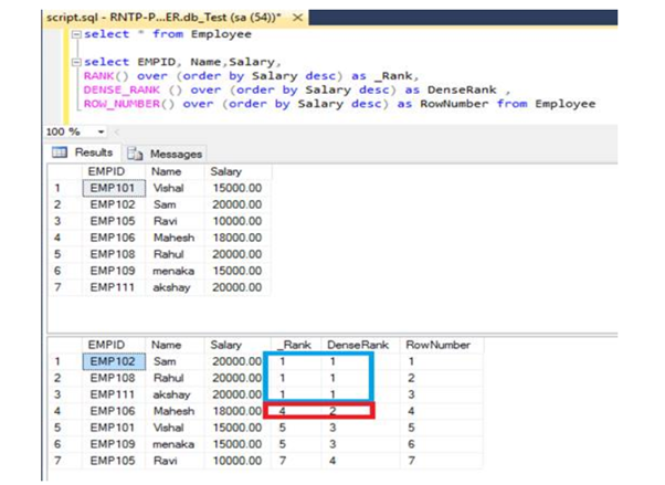
41. What is RANK, DANCE_RANK and ROW_NUMBER Functions?

Lets understand all terms with following example:

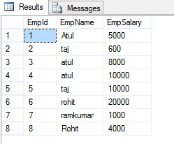
Here I have an Employe table, the following is the sample data for the Employe Table.
ROW_NUMBER() Function with Partition By clause:

The ROW_NUMBER() function assigns a unique sequential integer to rows within a partition of a result set. The numbering starts at 1 for the first row in each partition and increases by 1 for each subsequent row.

Syntax

ROW_NUMBER () OVER ([PARTITION BY value_exp, … [ n ]] ORDER BY_clause)

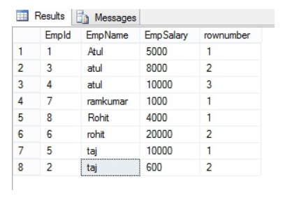
If we want to add row number to each group, partition by help to reset for every group, let’s take a look at the Employe table.

Select *, ROW_NUMBER() over(partition by Empname order by Empname ) as rownumber from Employee

The following is the OUTPUT of the above query
Rank() Function in SQL Server:

The RANK() function assigns a rank to rows based on the ordering of a specified column. Rows with the same value receive the same rank, and gaps are left in the ranking sequence for ties.

SELECT EmpName, EmpSalary ,rank() over(order by EmpName) as rankID from Employe;

The following is the OUTPUT of the above query.
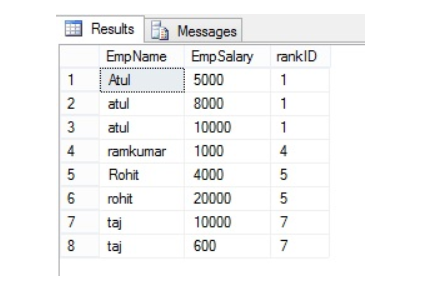
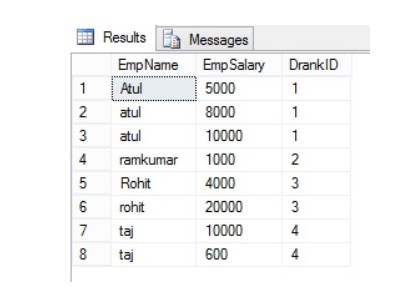
Gap represents number of occurrence example – EmpName=”atul” is repeated 3 times and has rank “1”, the next rank will be 1+3=4 and same with the next value.

Dense_Rank() Function in SQL Server:

The DENSE_RANK() function works similarly to RANK(), but it does not leave gaps in the ranking sequence when there are ties.

SELECT EmpName ,EmpSalary ,DENSE_RANK() over(order by EmpName) as DrankID from Employee

The following is the OUTPUT of the above query:
Summery:
42. Explain Normalization and De-Normalization.

Normalization and Denormalization are two opposite approaches in database design that impact how data is structured and managed:

1. Normalization:

Normalization is the process of organizing data in a database into multiple related tables to minimize redundancy and improve data integrity. The goal is to divide large tables into smaller, more manageable tables and establish relationships between them.

Key Features:

  • Reduces Data Redundancy: Data is broken down into multiple related tables to avoid duplication.
  • Improves Data Integrity: Reduces the chances of update, insert, and delete anomalies.
  • Follows Normal Forms: Data is structured according to various normal forms (1NF, 2NF, 3NF, etc.).
  • Optimized for Write Operations: It’s well-suited for transactional databases (OLTP) where data updates, inserts, and deletes are frequent.

Example:
Instead of storing both customer details and order details in a single table, normalization would separate them into two tables:

  • Customers Table: Contains customer information.
  • Orders Table: Contains order information with a foreign key reference to the Customers table.

2. Denormalization:

Denormalization is the process of combining related tables into one larger table to reduce the number of joins and improve read performance. It intentionally introduces redundancy for faster query performance.

Key Features:

  • Increases Redundancy: Some data is duplicated across tables, making reads faster.
  • Simplifies Queries: Fewer joins are needed, leading to improved performance for complex queries.
  • Optimized for Read Operations: It’s well-suited for analytical databases (OLAP) where read queries are frequent and need to be fast.
  • Data Integrity Challenges: With redundancy, maintaining consistency across data updates can be challenging.

Example:
In a denormalized database, customer and order details might be combined into a single table, avoiding the need for a join operation when querying both customer and order information.

Comparison:

FeatureNormalizationDenormalization
PurposeMinimize redundancy and maintain data integrityImprove read performance by reducing joins
Data StructureDivides data into multiple smaller tablesCombines data into fewer, larger tables
PerformanceOptimized for write operations (OLTP)Optimized for read operations (OLAP)
Data IntegrityHigh, with reduced redundancyLower, with potential data inconsistency issues
ComplexityRequires complex queries with multiple joinsSimplifies queries, often with less complex joins
Use CaseTransactional systems (e.g., banking, retail applications)Analytical systems (e.g., data warehouses, reporting)

Conclusion:

  • Normalization is used when data integrity and storage efficiency are priorities.
  • Denormalization is used when read performance is crucial, often at the cost of redundancy and potential data inconsistency.

In practice, the decision between normalization and denormalization depends on the specific needs of the application, whether it is more read-intensive or write-intensive, and the performance requirements.

43. What is a deadlock?

It is an unwanted situation where two or more transactions are waiting indefinitely for one another to release the locks. 

44. What is ALIAS command?

This command provides another name to a table or a column. It can be used in WHERE clause of a SQL query using the “as” keyword.

45. What is the difference between Datawarehouse, Data lake and lake house?

Here’s a comparison of a Data Warehouse, Data Lake, and Lakehouse:

FeatureData WarehouseData LakeLakehouse
PurposeStructured data storage for reporting and analysis.Store raw, unstructured, and semi-structured data.Combines features of both data warehouses and data lakes.
Data TypeStructured and relational data.Structured, semi-structured, and unstructured data.Supports structured, semi-structured, and unstructured data.
SchemaSchema-on-write (pre-defined schema).Schema-on-read (define schema when querying).Flexible schema handling (supports both schema-on-write and schema-on-read).
Data Storage FormatOptimized for tables and relational databases (e.g., SQL).Raw files in various formats (e.g., JSON, XML, Parquet).Stores data in formats like Parquet and Delta Lake with ACID properties.
Use CaseBI, reporting, and historical analysis on structured data.Big data analytics, data science, and exploratory analysis.Unified approach for BI, ML, and streaming analytics.
Processing EngineSQL-based processing (traditional OLAP).Supports multiple engines (e.g., Hadoop, Spark).Supports SQL, ML, and streaming engines in a unified platform.
Data GovernanceHigh control, with strict governance and data quality.Lower governance, flexible but with potential inconsistencies.Offers better governance and data quality control similar to data warehouses.
PerformanceHigh performance for structured queries and reports.May require optimization for specific queries.Optimized for both SQL analytics and large-scale data processing.
ScalabilityScales well for structured data but can be expensive.Highly scalable for any type of data, often cost-efficient.Scales efficiently, combining the benefits of both approaches.
CostCan be expensive due to compute and storage needs.Typically lower-cost storage, but processing can add cost.Cost-effective, combining cloud storage with optimized compute.
ExamplesAmazon Redshift, Snowflake, Google BigQuery.Amazon S3, Azure Data Lake, Hadoop HDFS.Databricks Lakehouse, Delta Lake, Google BigLake.

Summary:

  • Data Warehouses are best for structured data and traditional analytics.
  • Data Lakes are ideal for storing vast amounts of raw data for big data analytics and data science.
  • Lakehouses combine the strengths of both, offering a unified platform for various data types, supporting both traditional BI and advanced analytics.

46. What is OLTP?

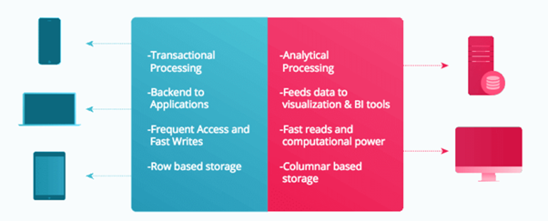
OLTP stands for Online Transaction Processing, is a class of software applications capable of supporting transaction-oriented programs. An essential attribute of an OLTP system is its ability to maintain concurrency. To avoid single points of failure, OLTP systems are often decentralized. These systems are usually designed for a large number of users who conduct short transactions. Database queries are usually simple, require sub-second response times and return relatively few records. Here is an insight into the working of an OLTP system.

47. What are the differences between OLTP and OLAP?

OLTP stands for Online Transaction Processing, is a class of software applications capable of supporting transaction-oriented programs. An important attribute of an OLTP system is its ability to maintain concurrency. OLTP systems often follow a decentralized architecture to avoid single points of failure. These systems are generally designed for a large audience of end users who conduct short transactions. Queries involved in such databases are generally simple, need fast response times and return relatively few records. Number of transactions per second acts as an effective measure for such systems.

OLAP stands for Online Analytical Processing, a class of software programs which are characterized by relatively low frequency of online transactions. Queries are often too complex and involve a bunch of aggregations. For OLAP systems, the effectiveness measure relies highly on response time. Such systems are widely used for data mining or maintaining aggregated, historical data, usually in multi-dimensional schemas.
48. What are the different Keys in relational Database?

In a relational database, various types of keys help define relationships, enforce integrity, and ensure data uniqueness. Here are the most commonly used keys:

Key TypeDescription
Primary KeyA unique identifier for each record in a table. It cannot contain NULL values.
Candidate KeyA set of attributes that can uniquely identify a record. The primary key is selected from candidate keys.
Super KeyA set of one or more attributes that can uniquely identify a record, possibly including extra attributes that are not needed for uniqueness.
Composite KeyA primary key consisting of more than one attribute (column). Used when no single attribute can uniquely identify records.
Foreign KeyAn attribute or a set of attributes in one table that refers to the primary key of another table, establishing a relationship between tables.
Unique KeyEnsures all values in a column or set of columns are unique. Unlike the primary key, it can contain NULL values.
Alternate KeyA candidate key that is not chosen as the primary key. Also known as a secondary key.
Surrogate KeyAn artificially generated key, usually a numeric value like an auto-incremented ID, used as a unique identifier. It has no business meaning and is only used internally.
Composite Foreign KeyA foreign key that consists of multiple columns, matching a composite primary key in another table.
Natural KeyA key that has a business meaning and is naturally present in the data (e.g., a Social Security Number or email address).
Key Definitions in Detail:
  1. Primary Key: Uniquely identifies each record in a table. A table can have only one primary key, which cannot have NULL values.
  2. Candidate Key: A set of attributes that can uniquely identify records. A table can have multiple candidate keys, but one of them becomes the primary key.
  3. Super Key: A combination of attributes that can uniquely identify records. Super keys can have extra, non-essential attributes.
  4. Composite Key: A key made up of two or more attributes to uniquely identify records.
  5. Foreign Key: A key used to link two tables, referencing the primary key in another table. It establishes referential integrity.
  6. Unique Key: Ensures uniqueness across rows in a column. It can have NULL values but ensures that all non-NULL values are unique.
  7. Alternate Key: A candidate key that was not selected as the primary key.
  8. Surrogate Key: An automatically generated unique key, often used in place of a natural key.
  9. Natural Key: A key that naturally exists in the data and has business relevance.

These keys play crucial roles in defining relationships, maintaining data integrity, and optimizing database performance.

49. What is LEAD and LAG function

The LEAD and LAG functions are analytic functions in SQL that allow you to access data from preceding or following rows within the same result set, without the need for self-joins. They are commonly used in data analysis for time-series data, rankings, and trends.

1. LAG Function:

The LAG function provides access to a value from a previous row (before the current row) in the same result set.

Syntax:

LAG(column_name, offset, default_value) OVER (PARTITION BY partition_column ORDER BY order_column)
  • column_name: The column from which you want to get the previous value.
  • offset: The number of rows back from the current row. The default is 1.
  • default_value: The value to return if there is no previous row (optional).
  • PARTITION BY: Divides the result set into partitions and applies the function within each partition.
  • ORDER BY: Determines the order of the rows within each partition.

Example:
Suppose you have a sales table with sales_id, sales_date, and amount. You want to see the previous day’s sales amount for each row.

SELECT
    sales_id,
    sales_date,
    amount,
    LAG(amount, 1, 0) OVER (ORDER BY sales_date) AS previous_day_amount
FROM
    sales;

This will show the amount from the previous day (row) next to the current day.

2. LEAD Function:

The LEAD function provides access to a value from the next row (after the current row) in the same result set.

Syntax:

LEAD(column_name, offset, default_value) OVER (PARTITION BY partition_column ORDER BY order_column)
  • column_name: The column from which you want to get the next value.
  • offset: The number of rows forward from the current row. The default is 1.
  • default_value: The value to return if there is no next row (optional).
  • PARTITION BY: Divides the result set into partitions and applies the function within each partition.
  • ORDER BY: Determines the order of the rows within each partition.

Example:
Using the same sales table, you want to see the next day’s sales amount for each row.

SELECT
    sales_id,
    sales_date,
    amount,
    LEAD(amount, 1, 0) OVER (ORDER BY sales_date) AS next_day_amount
FROM
    sales;

This will show the amount for the next day (row) next to the current day.

Use Cases:

  • LAG is useful for comparing a value with the previous period (e.g., sales growth compared to the previous month).
  • LEAD is useful for forecasting or seeing future trends (e.g., comparing current sales with next month’s expected sales).

Comparison Between LAG and LEAD:

  • LAG: Looks at the previous row.
  • LEAD: Looks at the next row.

Both functions are powerful tools in time-series analysis, trend detection, and data comparisons within partitions.

50. What is Left outer Join and Right Outer Join?

In SQL, LEFT OUTER JOIN and RIGHT OUTER JOIN are used to combine rows from two or more tables based on a related column between them. The key difference lies in how they handle rows that do not have matching data in both tables.

1. LEFT OUTER JOIN:

A LEFT OUTER JOIN (or simply LEFT JOIN) returns all records from the left table (Table A), and the matched records from the right table (Table B). If there is no match, NULL values are returned for columns from the right table.

Syntax:

SELECT columns
FROM table_A
LEFT OUTER JOIN table_B
ON table_A.column = table_B.column;

Behavior:

  • Includes all rows from the left table.
  • If there is no match in the right table, NULL values are displayed for columns from the right table.

Example:
Imagine you have two tables:

Customers Table (left table):

CustomerIDCustomerName
1Alice
2Bob
3Charlie

Orders Table (right table):

OrderIDCustomerIDOrderDate
10112024-08-01
10222024-08-03

Query:

SELECT Customers.CustomerID, Customers.CustomerName, Orders.OrderDate
FROM Customers
LEFT OUTER JOIN Orders
ON Customers.CustomerID = Orders.CustomerID;

Result:

CustomerIDCustomerNameOrderDate
1Alice2024-08-01
2Bob2024-08-03
3CharlieNULL

Here, Charlie has no matching order, so the OrderDate is NULL.

2. RIGHT OUTER JOIN:

A RIGHT OUTER JOIN (or simply RIGHT JOIN) returns all records from the right table (Table B), and the matched records from the left table (Table A). If there is no match, NULL values are returned for columns from the left table.

Syntax:

SELECT columns
FROM table_A
RIGHT OUTER JOIN table_B
ON table_A.column = table_B.column;

Behavior:

  • Includes all rows from the right table.
  • If there is no match in the left table, NULL values are displayed for columns from the left table.

Example:
Using the same Customers and Orders tables:

Query:

SELECT Customers.CustomerID, Customers.CustomerName, Orders.OrderDate
FROM Customers
RIGHT OUTER JOIN Orders
ON Customers.CustomerID = Orders.CustomerID;

Result:

CustomerIDCustomerNameOrderDate
1Alice2024-08-01
2Bob2024-08-03
NULLNULL2024-08-05

In this case, if there were an order in the Orders table that did not have a matching customer in the Customers table, it would still appear, with NULL values for CustomerID and CustomerName.

Key Differences:

AspectLEFT OUTER JOINRIGHT OUTER JOIN
Primary TableAll rows from the left table (Table A) are included.All rows from the right table (Table B) are included.
Matching RowsIncludes matching rows from the right table.Includes matching rows from the left table.
Unmatched RowsUnmatched rows from the left table appear with NULLs.Unmatched rows from the right table appear with NULLs.

Conclusion:

  • Use LEFT JOIN when you want to retain all rows from the left table.
  • Use RIGHT JOIN when you want to retain all rows from the right table.

These joins are useful in different scenarios depending on which table’s data you prioritize.

Reference:-

https://www.interviewbit.com

https://www.edureka.co
https://www.javatpoint.com

https://www.toptal.com/

https://hackr.io

https://www.mygreatlearning.com

https://www.guru99.com

https://www.edureka.co
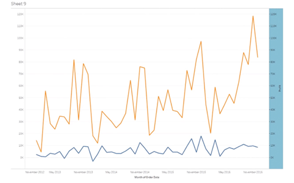
Tableau Interview Questions and answers

1. What is Tableau?

Tableau is a powerful data visualization tool used in the Business Intelligence Industry. It helps in simplifying raw data into a very easily understandable format.

2. What Are the Data Types Supported in Tableau?

Following data types are supported in Tableau:

  • Text (string) values
  • Date values
  • Date and time values
  • Numerical values
  • Boolean values (relational only)
  • Geographical values (used with maps)

3. How Will You Understand Dimensions and Measures?

DimensionsMeasures
Dimensions contain qualitative values (such as names, dates, or geographical data)Measures contain numeric, quantitative values that you can measure (such as Sales, Profit)
You can use dimensions to categorize, segment, and reveal the details in your data.Measures can be aggregated
Example: Category, City, Country, Customer ID, Customer Name, Order Date, Order IDExample: Profit, Quantity, Rank, Sales, Sales per Customer, Total Orders
  

4. What is Meant by ‘discrete’ and ‘continuous’ in Tableau?

The use of Tableau’s Discrete fields always results in headers being drawn whenever they are placed on the Rows or Columns shelves. On the other hand, Tableau Continuous fields always result in axes when you add them to the view. 

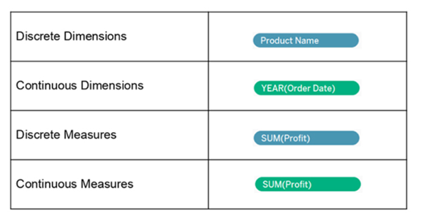
Continuous in Tableau will give you an overall trend of the data that you are looking at. While Discrete in Tableau allows you to segment the data to analyze it in different ways. Moreover, Tableau’s Discrete function gives you the chance to take something that would be the cumulative total of something and break it down into segments or chunks and see your data in different ways. This is not something that Excel can easily do. Changing these can affect how you present information. Discrete data in Tableau is always represented with a blue pill on the shelf, while Continuous data in Tableau is always green. 

  • Discrete – “individually separate and distinct.”
  • Continuous – “forming an unbroken whole without interruption.”

The values are as shown:

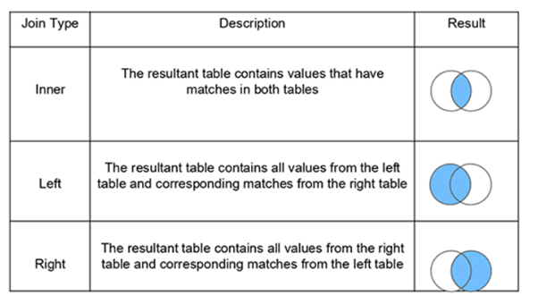
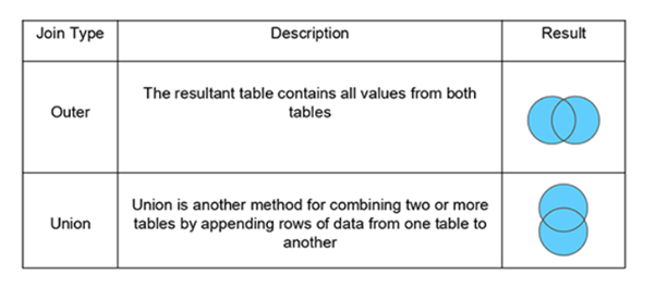
5. What Are the Different Joins in Tableau?

Joining is a method for combining related data on a common key. Below is a table that lists the different types of joins:

6. What is the Difference Between a Live Connection and an Extract?

Tableau Data Extracts are snapshots of data optimized for aggregation and loaded into system memory to be quickly recalled for visualization.

Example: Hospitals that monitor incoming patient data need to make real-time decisions.

Live connections offer the convenience of real-time updates, with any changes in the data source reflected in Tableau.

Example: Hospitals need to monitor the patient’s weekly or monthly trends that require data extracts.

Note:-

When you create an extract of the data, Tableau doesn’t need access to the database to build the visualization, so processing is faster.

If you have a Tableau server, the extract option can be set to a refresh schedule to be updated. 

7. What is a Calculated Field, and How Will You Create One?

A calculated field is used to create new (modified) fields from existing data in the data source. It can be used to create more robust visualizations and doesn’t affect the original dataset.

For example, let’s calculate the “average delay to ship.”

The data set considered here has information regarding order date and ship date for four different regions. To create a calculated field:

  1. Go to Analysis and select Create Calculated Field. 
  2. A calculation editor pops up on the screen. Provide a name to the calculated field: Shipping Delay.
  3. Enter the formula: DATEDIFF (‘day’, [Order Date], [Ship Date])
  4. Click on Ok.
  5. Bring Shipping Delay to the view.
  6. Repeat steps 1 to 5 to create a new calculated field ‘Average Shipping Delay’ using the formula: AVG (DATEDIFF (‘day,’ [Order Date], [Ship Date]))

7. Drag Region field to Rows shelf and SUM(Average Shipping Delay) to the marks card; the average delay for each region gets displayed.

8.  How Can You Display the Top Five and Bottom Five Sales in the Same View?

We can display it using the In/Out functionality of sets.

Follow these steps:

  1. Drag the Customer Name field to Rows shelf and Profit field to Columns shelf to get the visualization.
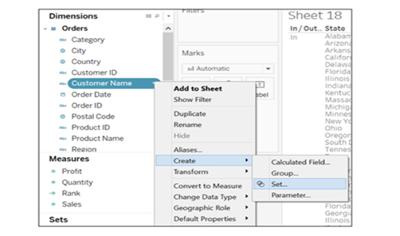
  2. Create a set by right-clicking on the Customer Name field. Choose to create an option and click on Set.
  3. Provide the name ‘Top Customers’ to the set. Configure the set by clicking on Top tab, selecting By field, and filling the values as Top, 5, Profit, and Sum. 
  4. Similarly, create a second set called ‘Bottom Customers’ and fill the By Field values as Bottom, 5, Profit, and Sum. 
  5. Select these two sets and right-click on it. Use the option Create Combined Set. Name it ‘Top and Bottom Customers’ and include all members of both sets. Pull the Top and Bottom Customers onto Filters

The top five and bottom five are displayed:

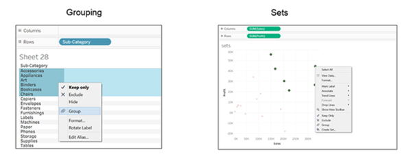
9. Is There a Difference Between Sets and Groups in Tableau?

A Tableau group is one dimensional, used to create a higher level category by using lower-level category members. Tableau sets can have conditions and can be grouped across multiple dimensions/measures.

Example: Sub-category can be grouped by category.

Top Sales and profit can be clubbed together for different categories by creating a set:

  1. Continuing with the above example of Sets, select the Bottom Customers set where customer names are arranged based on profit. 
  2. Go to the ‘Groups’ tab and select the top five entries from the list. 
  3. Right-click and select create a group option. 
  4. Similarly, select the bottom five entries and create their group. Hide all the other entries.

A key difference here is that the groups will consist of the same customers even if their profits change later. While for sets, if the profit changes, the top five and bottom five customers will change accordingly.

Note-

We can’t use groups in calculated fields, but we can use sets.

10.  What is the Difference Between Treemaps and Heat Maps?

Heat Maps

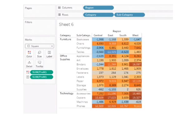
A Heat map is used to compare categories using color and size. In this, we can distinguish two measures.

Scenario: Show sales and profit in all regions for different product categories and sub-categories.

Follow these steps:

  1. Drag Region field to Columns shelf, and Category and Sub-Category fields in Rows shelf. 
  2. Use the ShowMe tool and select the Heat Map.
  3. Observe the hotter and colder regions in the heat map produced:

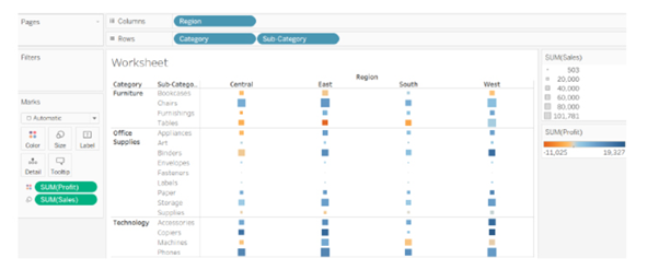
A heat map is not only defined by color, but you can also use its size. Here we define the size by sale by dragging the Sales tab to Size under marks card, comparing profit and sales through the color and size.

Analysis: Profit is represented by color and ranges from orange for loss to blue for profit. The total sales are represented by size.

Tree Maps

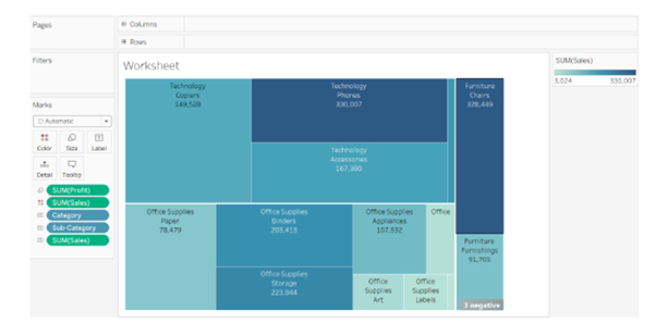
A Treemap is used to represent hierarchical data. The space in the view is divided into rectangles that are sized and ordered by a measure. Scenario: Show sales and profit in all regions for different product categories and sub-categories.

  1. Select two dimensions Category and Sub-Category
  2. Select two measures Sales and Profit from the data pane. 
  3. Use the Show-me tool and select tree-map.

This is how it looks:

Analysis: The larger the size of the node, the higher the profit in that category. Similarly, the darker the node, the more sales in that category.

.twbx

The .twbx contains all of the necessary information to build the visualization along with the data source. This is called a packaged workbook, and it compresses the package of files altogether.

.twb

The .twb contains instructions about how to interact with the data source. When it’s building a visualization, Tableau will look at the data source and then build the visualization with an extract. It can’t be shared alone as it contains only instructions, and the data source needs to be attached separately.

11. Explain the Difference Between Tableau Worksheet, Dashboard, Story, and Workbook?

  • Tableau uses a workbook and sheet file structure, much like Microsoft Excel.
  • A workbook contains sheets, which can be a worksheet, dashboard, or a story.
  • A worksheet contains a single view along with shelves, legends, and the Data pane.
  • A dashboard is a collection of views from multiple worksheets.
  • A story contains a sequence of worksheets or dashboards that work together to convey information.

12. What Do You Understand the Blended Axis?

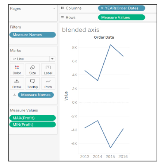
Blended Axis is used to blend two measures that share an axis when they have the same scale. 

Scenario: Show Min and Max profit in the same pane and have a unified axis for both, so that it is quicker and easier to interpret the chart.

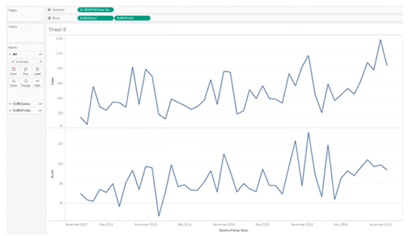
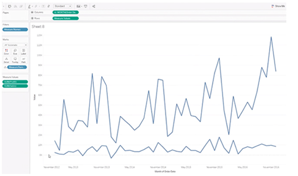
First, create a visualization that shows sales over time. Next, see profit along with sales over the same time. Here, you get two visualizations, one for sales over time and the other for-profit over time.

To see a visualization that has a blended axis for sales over time and profit over time, we bring in Measure Values and select the properties that we want to keep (Sales and Profit), removing all of the rest. You can now see profit and sales over one blended axis.

13. What is the Use of Dual-axis? How Do You Create One?

Dual Axis allows you to compare measures, and this is useful when you want to compare two measures that have different scales.

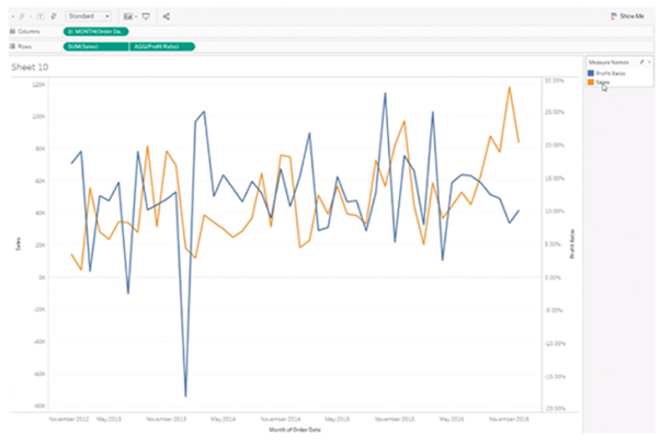
Considering the same example used in the above question, first create a visualization with sales over time and profit over time. To create a dual-axis, right-click on the second pill of the measures and select Dual Axis.

Observe that sales and profit do not share the same axis, and profit is much higher towards the end. 

The difference between a blended axis and a dual-axis chart is that the blended axis uses the same scale, while a dual-axis could have two different scales and two marks cards.

Scenario: We want to show Sales by year and Profit Ratio by year in the same view.

We create a visualization of sales over time and profit ratio over time. Observe that sales and profit ratio can’t use the same scale as the profit ratio is in percentage. As we want the two parameters in the same area, we right-click on Profit Ratio and select Dual Axis.

14. What is the Rank Function in Tableau?

The ranking is assigning something a position usually within a category and based on a measure. Tableau can rank in several ways like:

  • rank 
  • rank_dense
  • rank_modified 
  • rank_unique

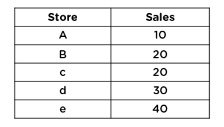
Consider five stores whose sales are as shown:

Let us understand how they are ranked based on their sales:

  1. Drag Store field to Rows shelf and Sales field to the marks card. 
  2. Create a Calculated Field named Rank and use the formula: RANK (SUM(Sales))
  3. Bring the Rank field to the marks card.
  4. Double-click on the Rank field, and you can see the rank assigned to the stores based on sales. 

Next, duplicate the Rank field by right-clicking on it and selecting Duplicate. Name the copy as ‘Rank Modified’ and use the formula:

RANK MODIFIED (SUM(Sales))

Bring Rank Modified to the marks card to view the data. 

Repeat the same steps to create ‘Rank Dense’ and use the formula:

RANK DENSE (SUM(Sales)) 

Similarly, create ‘Rank Unique’ and use the formula:

RANK UNIQUE (SUM(Sales)) 

15. How Do You Handle Null and Other Special Values?

If the field contains null values or if there are zeros or negative values on a logarithmic axis, Tableau cannot plot them. Tableau displays an indicator in the lower right corner of the view, and you can click the indicator and choose from the following options:

  • Filter Data
    Excludes the null values from the visualization using a filter. In that case, the null values are also excluded from any calculations used in the view.
  • Show Data at Default Position
    Shows the data at a default location on the axis.

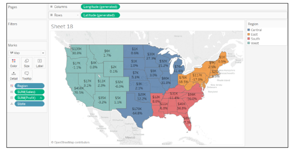
16. Design a View to Show Region Wise Profit and Sales.

Follow these simple steps to show region wise profit and sales:

  1. Drag Profit and Sales field to the Rows shelf
  2. Drag Region field to the Columns shelf

But for such questions, the interviewer may be looking for your mapping capabilities in Tableau. 

So, you need to follow these steps to show region wise profit and sales in a better way:

  1. Double click on the State field to get its view
  2. Go to Marks card and change the mark type from Automatic to Map.
  3. Bring Region field to Color on the Marks card
  4. Drag Profit, Sales, and State fields to Label on the Marks card

These steps produce a better view of region-wise profit and sales, as shown:

17. How Can You Optimize the Performance of a Dashboard?

There are multiple ways to optimize the performance of the dashboard like:

  • Maximize the number of fields and records. You can exclude unused fields from your visualization or use extract filters.
  • Limit the number of filters used, by avoiding quick filters and using action and parameter filters instead. These filters reduce query loads. 
  • use Min/Max instead of Average because average functions require more processing time than Min/Max
  • Use boolean or numerical calculations more than string calculations. Computers can process integers and boolean much faster than strings.

Boolean > int > float > date-time > string

18. What are the different kinds of filters in Tableau?

Tableau offers a good range of filters that we can apply on the data for better analysis.

Filters allow us to view our data at different levels of granularity and detail. We can exclude unnecessary data through filters and conduct our analysis on only the required data. There are five different types of filters available in Tableau.

1. Extract filters: These filters create an extract or subset of data from the original data source.

In other words, the extract filters extract a portion of data from the whole from its source. We can use the data extract anywhere in the analysis once it is created.

2. Data Source filters: The data source filters are the filter conditions that we can directly apply at the data source level.

Using the data source filters we can apply filters on the data present in the data source itself instead of first importing it into Tableau.

3. Context filters: The context filters are used to apply a context for the data that we are working on.

Once we apply a context filter on a worksheet or workbook, the entire analysis is done in that applied context only.

4. Dimension filters: Dimension filters are applied specifically on individual dimensions present in the Dimensions section on a Tableau sheet.

We can easily apply dimension filters on the dimension fields by dragging and dropping the field into the Filter card present on the sheet.

5. Measure filters: Such filters are applied on individual measure fields present in the Measures section on a Tableau sheet.

We can easily apply the measure filters on the measure fields by dragging and dropping the field into the Filter card present on the sheet.

19. What do you understand by context filters?

Context filters are used to apply context on the data under analysis.

By applying a context we set a perspective according to which we can see the charts and graphs.

For example, we have sales data of an electronic store and we want to conduct our analysis only for the corporate sector or segment.

To do this, we have to apply a context filter on our Tableau sheet. Once we add the context for the Corporate segment from the Add to context option, all the charts present on the sheet will only show data relevant to the Corporate segment.

In this way, we can apply a context to our analysis in Tableau.

20. What is Quick Sorting in Tableau?

Tableau gives us the option to Quick Sort data present in our visualizations.

We can instantly sort data from the visualization by simply clicking on the sort button present on the axes of a graph or chart.

An ascending sort is performed upon one click, the descending sort is performed on two clicks and an applied sort is cleared on three clicks on the Quick Sort icon.

21. What is Data Blending in Tableau?

Consider the same client. Suppose, they are operating their services in Asia, Europe, NA, and so on, and they are maintaining Asia data in SQL, Europe data in SQL Server, and NA data in MySQL.

Now, our client wants to analyze their business across the world in a single worksheet. In this case, we can’t perform a Join. Here, we have to make use of the data blending concept.

Normally, in Tableau, we can perform the analysis on a single data server. If we want to perform the analysis of data from multiple data sources in a single sheet, then we have to make use of this new concept called data blending.

Data blending mixes the data from different data sources and allows users to perform the analysis in a single sheet. ‘Blending’ means ‘mixing’ and when we are mixing the data sources, then it is called data blending.

Rules to Perform Data Blending

In order to perform data blending, there are a few rules:

  • If we are performing data blending on two data sources, these two data sources should have at least one common dimension.
  • In that common dimension, at least one value should be matching.

In Tableau, we can perform data blending in two ways.

  • Automatic way: Here, Tableau automatically defines the relationship between the two data sources based on the common dimensions and based on the matching values, and the relationship is indicated in orange.
  • Custom or Manual way: In the manual or custom way, the user needs to define the relationship manually.

Data Blending Functionality

  • All the primary and secondary data sources are linked by a specific relationship.
  • While performing data blending, each worksheet has a primary connection, and optionally it might contain several secondary connections.
  • All the primary connections are indicated in blue in the worksheet and all the secondary connections with an orange-colored tick mark.
  • In data blending, one sheet contains one primary data source and it can contain n number of secondary data sources.

22. What is the use of the new custom SQL query in Tableau?

Custom SQL query is written after connecting to data for pulling the data in a structured view. For example, suppose, we have 50 columns in a table, but we need just 10 columns only. So instead of taking 50 columns, we can write a SQL query. The performance will increase.

23. How to create cascading filters without using context filter?

Here, say, we have Filter1 and Filter2. Based on Filter1, we need to use Filter2 on the data. For example, consider Filter1 as ‘Country’ and Filter2 as ‘States.’

Let’s choose Country as ‘India’ and hence Filter2 should display only the states of India. Choose options of Filter2 states: select option of ‘Only relevant values’

24. How can we combine a database and the flat file data in Tableau Desktop?

Connect data twice, once for database tables and then for the flat file. The Data->Edit Relationships

Give a Join condition on the common column from DB tables to the flat file.

25. How will you publish and schedule a workbook in Tableau Server?

First, create a schedule for a particular time and then create Extract for the data source and publish the workbook on the server.

Before we publish it, there is an option called ‘Scheduling and Authentication’. Click on that and select the schedule from the drop-down and then publish. Also publish data source and assign the schedule. This schedule will automatically run for the assigned time and the workbook will get refreshed on a regular basis.

26. Distinguish between Parameters and Filters.

Parameters are dynamic values that can replace constant values in calculations. Parameters can serve as Filters as well.

Filters, on the other hand, are used to restrict the data based on a condition that we have mentioned in the Filters shelf.

27. How to view a SQL generated by Tableau Desktop?

Tableau Desktop Log files are located in C:/Users/MyDocuments/My Tableau Repository. If we have a live connection to the data source, we need to check the log.txt and tabprotosrv.txt files. If we are using Extract, have to check the tdeserver.txt file. The tabprotosrv.txt file often shows detailed information about queries.

28. What are the five main products offered by Tableau?

Tableau offers five main products:

  • Tableau Desktop
  • Tableau Server
  • Tableau Online
  • Tableau Reader
  • Tableau Public

Tableau Desktop

Tableau Desktop has a rich feature set and allows you to code and customize reports. It ables users to create charts, reports, and dashboards.

Tableau Public

It is the Tableau version specially build for cost-effective users. By the word “Public,” it means that the workbooks created cannot be saved locally. In turn, it should be saved to Tableau’s public cloud, which can be viewed and accessed by anyone.

Tableau Server

The software is specifically used to share the workbooks, visualizations that are created in the Tableau Desktop application across the organization.

Tableau Online

As the name suggests, it is an online sharing tool for Tableau. Its functionalities are similar to Tableau Server, but the data is stored on servers hosted in the cloud, which are maintained by the Tableau group.

Tableau Reader

Tableau Reader is a free tool that enables the user to view the workbooks and visualizations created using Tableau Desktop or Tableau Public. The data can be filtered, but editing and modifications are restricted. The security level is zero in Tableau Reader as anyone who gets the workbook can view it using Tableau Reader.

29. What are the advantages of Using Context Filters?

The advantages of Using Context Filters

  • Improve Performance: When context filter is used in large data sources, it can improve the performance as it creates a temporary dataset part based on the context filter selection. The performance can be effectively improved through the selection of major categorical context filters.
  • Dependent Filter Conditions: Context filters can be used to create dependent filter conditions based on the business requirement. When the data source size is large, context filters can be selected on the primary category, and other relevant filters can be executed.

30. Explain story in Tableau

A story is a sheet containing a dashboard or worksheet sequence that works together to convey particular information.

31. Distinguish between Treemaps and Heat Maps

TreeMapHeat Map
TreeMap represents and shows data hierarchically as a group of nested rectangles.Heat Map represents the data graphically with multiple colors to represent values.
It can be used for comparing the categories with size, colors, and illustrating the hierarchical data.It can be used for comparing the categories depend on size and color.

32. Explain data modelling

Data modeling (data modeling) is the process of creating a data model for the data to be stored in a database.

This data model is a conceptual representation of Data objects, the associations between different data objects, and the rules. Data modeling helps in the visual representation of data and enforces business rules, regulatory compliances, and government policies on the data.

33. Name the components of a Dashboard.

Important components of a Dashboard are:

  • Horizontal: A horizontal layout allows the designer to group dashboard components and worksheets across the page.
  • Vertical: Vertical containers enables the user to group dashboard components and worksheets top to bottom down your page. It also allows users to edit the width of all elements at once.
  • Text: It contains all textual files
  • Image Extract: Tableau applies some code to extract the image that is stored in XML.
  • URL action: It is a hyperlink that points to file, web page, or other web-based resources.

34. What are the different Types of Graphs and Charts for Presenting Data?

To better understand each chart and how they can be used, here’s an overview of each type of chart.

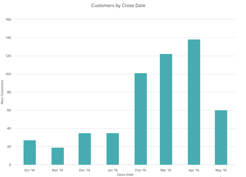
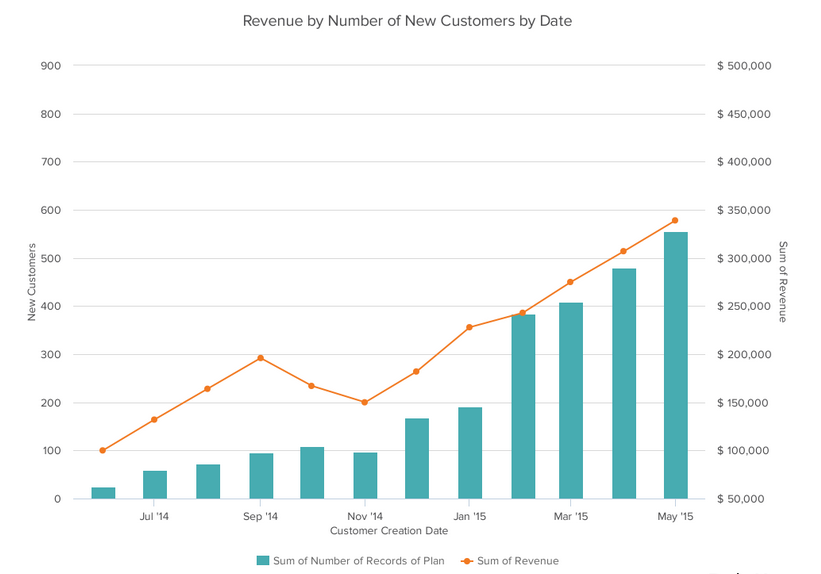
1. Column Chart:

A column chart is used to show a comparison among different items, or it can show a comparison of items over time. You could use this format to see the revenue per landing page or customers by close date.

Image Source: blog.hubspot.com

Design Best Practices for Column Charts:

  • Use consistent colors throughout the chart, selecting accent colors to highlight meaningful data points or changes over time.
  • Use horizontal labels to improve readability.
  • Start the y-axis at 0 to appropriately reflect the values in your graph.

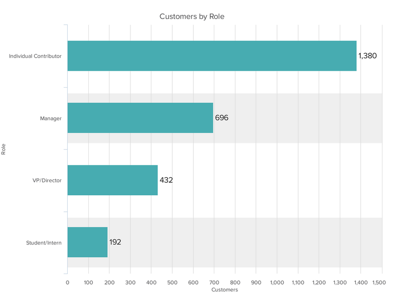
2. Bar Graph:

A bar graph, basically a horizontal column chart, should be used to avoid clutter when one data label is long or if you have more than 10 items to compare. This type of visualization can also be used to display negative numbers.

Design Best Practices for Bar Graphs:

  • Use consistent colors throughout the chart, selecting accent colors to highlight meaningful data points or changes over time.
  • Use horizontal labels to improve readability.
  • Start the y-axis at 0 to appropriately reflect the values in your graph.

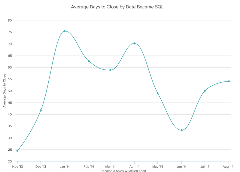
3. Line Graph:

A line graph reveals trends or progress over time and can be used to show many different categories of data. You should use it when you chart a continuous data set.

Design Best Practices for Line Graphs:

  • Use solid lines only.
  • Don’t plot more than four lines to avoid visual distractions.
  • Use the right height so the lines take up roughly 2/3 of the y-axis’ height.

4. Dual Axis Chart:

A dual axis chart allows you to plot data using two y-axes and a shared x-axis. It’s used with three data sets, one of which is based on a continuous set of data and another which is better suited to being grouped by category. This should be used to visualize a correlation or the lack thereof between these three data sets.

Design Best Practices for Dual Axis Charts:

  • Use the y-axis on the left side for the primary variable because brains are naturally inclined to look left first.
  • Use different graphing styles to illustrate the two data sets, as illustrated above.
  • Choose contrasting colors for the two data sets.

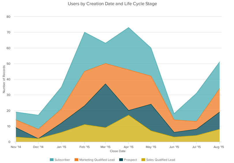
5. Area Chart:

An area chart is basically a line chart, but the space between the x-axis and the line is filled with a color or pattern. It is useful for showing part-to-whole relations, such as showing individual sales reps’ contribution to total sales for a year. It helps you analyze both overall and individual trend information.

Design Best Practices for Area Charts:

  • Use transparent colors so information isn’t obscured in the background.
  • Don’t display more than four categories to avoid clutter.
  • Organize highly variable data at the top of the chart to make it easy to read.

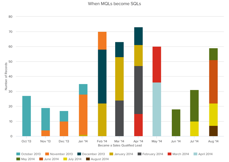
6. Stacked Bar Chart:

This should be used to compare many different items and show the composition of each item being compared.

Design Best Practices for Stacked Bar Graphs:

  • Best used to illustrate part-to-whole relationships.
  • Use contrasting colors for greater clarity.
  • Make chart scale large enough to view group sizes in relation to one another.

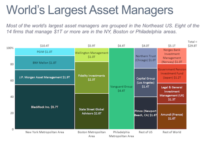
7. Mekko Chart:

Also known as a marimekko chart, this type of graph can compare values, measure each one’s composition, and show how your data is distributed across each one.

It’s similar to a stacked bar, except the mekko’s x-axis is used to capture another dimension of your values — rather than time progression, like column charts often do. In the graphic below, the x-axis compares each city to one another.

Design Best Practices for Mekko Charts:

  • Vary you bar heights if the portion size is an important point of comparison.
  • Don’t include too many composite values within each bar. you might want to reevaluate how to present your data if you have a lot. 
  • Order your bars from left to right in such a way that exposes a relevant trend or message.

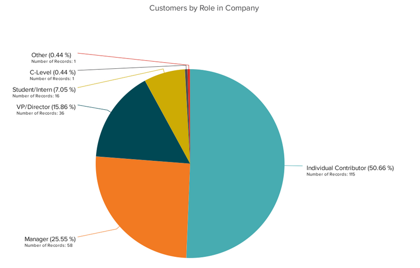
8. Pie Chart:

A pie chart shows a static number and how categories represent part of a whole — the composition of something. A pie chart represents numbers in percentages, and the total sum of all segments needs to equal 100%.

Design Best Practices for Pie Charts:

  • Don’t illustrate too many categories to ensure differentiation between slices.
  • Ensure that the slice values add up to 100%.
  • Order slices according to their size.

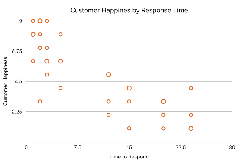
9. Scatter Plot Chart:

A scatter plot or scattergram chart will show the relationship between two different variables or it can reveal the distribution trends. It should be used when there are many different data points, and you want to highlight similarities in the data set. This is useful when looking for outliers or for understanding the distribution of your data.

Design Best Practices for Scatter Plots:

  • Include more variables, such as different sizes, to incorporate more data.
  • Start y-axis at 0 to represent data accurately.
  • If you use trend lines, only use a maximum of two to make your plot easy to understand.

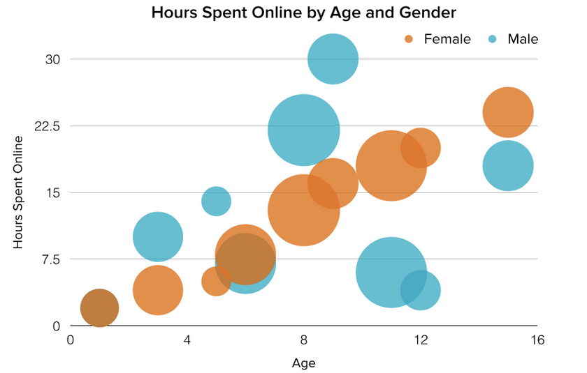
10. Bubble Chart:

A bubble chart is similar to a scatter plot in that it can show distribution or relationship. There is a third data set, which is indicated by the size of the bubble or circle.

Design Best Practices for Bubble Charts:

  • Scale bubbles according to area, not diameter.
  • Make sure labels are clear and visible.
  • Use circular shapes only.

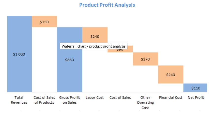
11. Waterfall Chart:

A waterfall chart should be used to show how an initial value is affected by intermediate values — either positive or negative — and resulted in a final value. This should be used to reveal the composition of a number. An example of this would be to showcase how overall company revenue is influenced by different departments and leads to a specific profit number.

Design Best Practices for Waterfall Charts:

  • Use contrasting colors to highlight differences in data sets.
  • Choose warm colors to indicate increases and cool colors to indicate decreases.

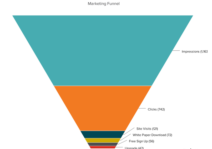
12. Funnel Chart:

Design Best Practices for Funnel Charts:

  • Scale the size of each section to accurately reflect the size of the data set.
  • Use contrasting colors or one color in gradating hues, from darkest to lightest as the size of the funnel decreases.

13. Bullet Graph:

A bullet graph reveals progress toward a goal, compares this to another measure, and provides context in the form of a rating or performance.

Design Best Practices for Bullet Graphs:

  • Use contrasting colors to highlight how the data is progressing.
  • Use one color in different shades to gauge progress.

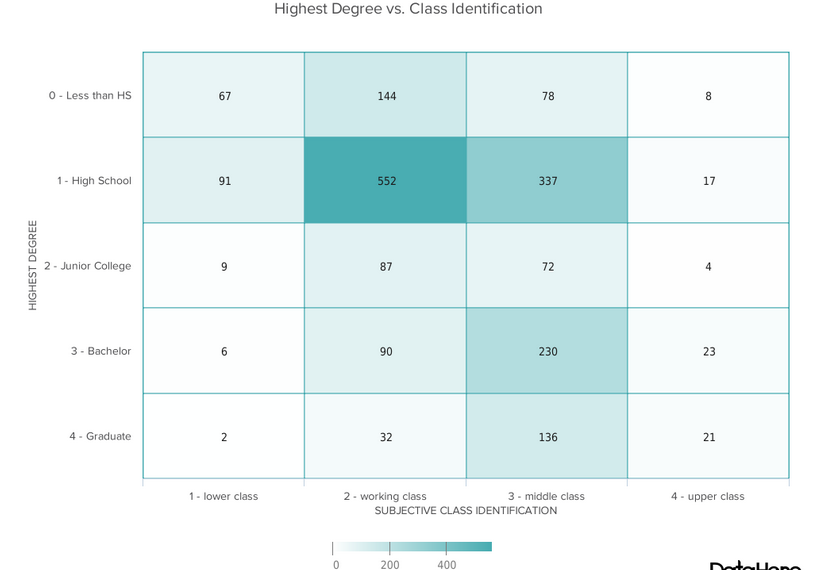
14. Heat Map:

A heat map shows the relationship between two items and provides rating information, such as high to low or poor to excellent. The rating information is displayed using varying colors or saturation.

Image source: blog.hubspot.com

Design Best Practices for Heat Map:

  • Use a basic and clear map outline to avoid distracting from the data.
  • Use a single color in varying shades to show changes in data.
  • Avoid using multiple patterns.

Reference:

  1. www.simplilearn.com
  2. https://data-flair.training
  3. https://www.edureka.co
  4. https://intellipaat.com
  5. https://intellipaat.com

Machine Leaning interview questions and answers

1. What is Data Science?

Data Science is a combination of algorithms, tools, and machine learning technique which helps you to find common hidden patterns from the given raw data.

2. What are the differences between supervised and unsupervised learning?

Supervised LearningUnsupervised Learning
Uses known and labeled data as inputUses unlabeled data as input
Supervised learning has a feedback mechanismUnsupervised learning has no feedback mechanism 
The most commonly used supervised learning algorithms are decision trees, logistic regression, and support vector machineThe most commonly used unsupervised learning algorithms are k-means clustering, hierarchical clustering, and apriori algorithm
  

3. What do you understand by linear regression?

Linear regression helps in understanding the linear relationship between the dependent and the independent variables. Linear regression is a supervised learning algorithm, which helps in finding the linear relationship between two variables. One is the predictor or the independent variable and the other is the response or the dependent variable. In Linear Regression, we try to understand how the dependent variable changes w.r.t the independent variable. If there is only one independent variable, then it is called simple linear regression, and if there is more than one independent variable then it is known as multiple linear regression.

4. How do you find RMSE and MSE in a linear regression model?

RMSE and MSE are two of the most common measures of accuracy for a linear regression model.  RMSE indicates the Root Mean Square Error. 

MSE indicates the Mean Square Error.

5. How is logistic regression done?

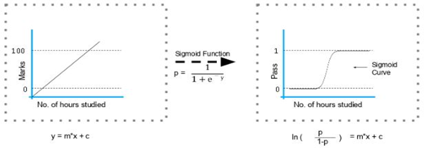
Logistic regression measures the relationship between the dependent variable (our label of what we want to predict) and one or more independent variables (our features) by estimating probability using its underlying logistic function (sigmoid).

The image shown below depicts how logistic regression works:

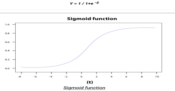
The formula and graph for the sigmoid function are as shown:

6. What is the Sigmoid Function?

It is a mathematical function having a characteristic that can take any real value and map it to between 0 to 1 shaped like the letter “S”. The sigmoid function also called a logistic function.

So, if the value of z goes to positive infinity then the predicted value of y will become 1 and if it goes to negative infinity then the predicted value of y will become 0. And if the outcome of the sigmoid function is more than 0.5 then we classify that label as class 1 or positive class and if it is less than 0.5 then we can classify it to negative class or label as class 0.

7. Why do we use the Sigmoid Function?

Sigmoid Function acts as an activation function in machine learning which is used to add non-linearity in a machine learning model, in simple words it decides which value to pass as output and what not to pass.

8. How will you explain linear regression to a non-tech person?

Linear Regression is a statistical technique of measuring the linear relationship between the two variables. By linear relationship, we mean that an increase in a variable would lead to increase in the other variable and a decrease in one variable would lead to attenuation in the second variable as well. Based on this linear relationship, we establish a model that predicts the future outcomes based on an increase in one variable.

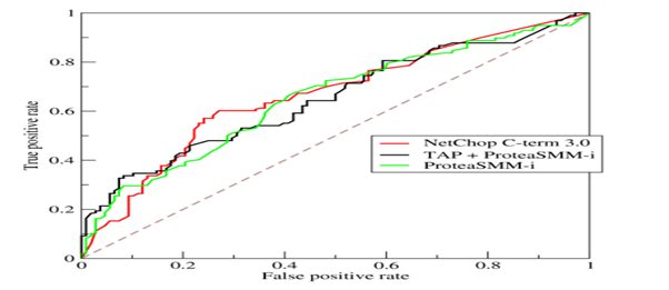
9. Explain how a ROC curve works?

The ROC curve is a graphical representation of the contrast between true positive rates and false-positive rates at various thresholds. It is often used as a proxy for the trade-off between the sensitivity (true positive rate) and false-positive rate

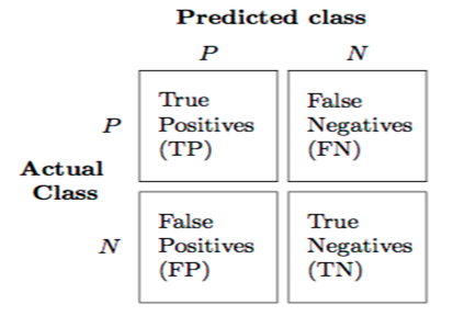
10. What is Precision, Recall, Accuracy and F1-score?

Once you have built a classification model, you need evaluate how good the predictions made by that model are. So, how do you define ‘good’ predictions?

There are some performance metrics which help us improve our models. Let us explore the differences between them for a binary classification problem:

Consider the following Confusion Matrix for a classification problem which predicts whether a patient has Cancer or not for 100 patients:

Now, the following are the fundamental metrics for the above data:

Precision: It is implied as the measure of the correctly identified positive cases from all the predicted positive cases. Thus, it is useful when the costs of False Positives is high.

Recall: It is the measure of the correctly identified positive cases from all the actual positive cases. It is important when the cost of False Negatives is high.

Accuracy: One of the more obvious metrics, it is the measure of all the correctly identified cases. It is most used when all the classes are equally important.

Now for our above example, suppose that there only 30 patients who actually have cancer. What if our model identifies 25 of those as having cancer?

The accuracy in this case is = 90% which is a high enough number for the model to be considered as ‘accurate’. However, there are 5 patients who actually have cancer and the model predicted that they don’t have it. Obviously, this is too high a cost. Our model should try to minimize these False Negatives. For these cases, we use the F1-score.

F1-score: This is the harmonic mean of Precision and Recall and gives a better measure of the incorrectly classified cases than the Accuracy Metric.

We use the Harmonic Mean since it penalizes the extreme values.

To summaries the differences between the F1-score and the accuracy,

  • Accuracy is used when the True Positives and True negatives are more important while F1-score is used when the False Negatives and False Positives are crucial
  • Accuracy can be used when the class distribution is similar while F1-score is a better metric when there are imbalanced classes as in the above case.
  • In most real-life classification problems, imbalanced class distribution exists and thus F1-score is a better metric to evaluate our model on.

11. How is AUC different from ROC?

AUC curve is a measurement of precision against the recall. Precision = TP/(TP + FP) and TP/(TP + FN). This is in contrast with ROC that measures and plots True Positive against False positive rate.

12. What is Selection Bias?

Selection bias is a kind of error that occurs when the researcher decides who is going to be studied. It is usually associated with research where the selection of participants isn’t random. It is sometimes referred to as the selection effect. It is the distortion of statistical analysis, resulting from the method of collecting samples. If the selection bias is not taken into account, then some conclusions of the study may not be accurate.

The types of selection bias include:

  1. Sampling bias: It is a systematic error due to a non-random sample of a population causing some members of the population to be less likely to be included than others resulting in a biased sample.
  2. Time interval: A trial may be terminated early at an extreme value (often for ethical reasons), but the extreme value is likely to be reached by the variable with the largest variance, even if all variables have a similar mean.
  3. Data: When specific subsets of data are chosen to support a conclusion or rejection of bad data on arbitrary grounds, instead of according to previously stated or generally agreed criteria.
  4. Attrition: Attrition bias is a kind of selection bias caused by attrition (loss of participants) discounting trial subjects/tests that did not run to completion

13. Differentiate between uni-variate, bi-variate, and multivariate analysis

Univariate:

Univariate data contains only one variable. The purpose of the univariate analysis is to describe the data and find patterns that exist within it.

Example: height of students.

The patterns can be studied by drawing conclusions using mean, median, mode, dispersion or range, minimum, maximum, etc.

Bivariate:

Bivariate data involves two different variables. The analysis of this type of data deals with causes and relationships and the analysis is done to determine the relationship between the two variables.

Example: temperature and ice cream sales in the summer season. Here, the relationship is visible from the table that temperature and sales are directly proportional to each other. The hotter the temperature, the better the sales.

Multivariate:

Multivariate data involves three or more variables, it is categorized under multivariate. It is similar to a bivariate but contains more than one dependent variable. Example: data for house price prediction. The patterns can be studied by drawing conclusions using mean, median, and mode, dispersion or range, minimum, maximum, etc. You can start describing the data and using it to guess what the price of the house will be.

14. Explain the steps in making a decision tree.

Following are the steps:
  • Step-1: Begin the tree with the root node, says S, which contains the complete dataset.
  • Step-2: Find the best attribute in the dataset using Attribute Selection Measure (ASM).
  • Step-3: Divide the S into subsets that contains possible values for the best attributes.
  • Step-4: Generate the decision tree node, which contains the best attribute.
  • Step-5: Recursively make new decision trees using the subsets of the dataset created in step -3. Continue this process until a stage is reached where you cannot further classify the nodes and called the final node as a leaf node.

For example, let’s say you want to build a decision tree to decide whether you should accept or decline a job offer. The decision tree for this case is as shown:

It is clear from the decision tree that an offer is accepted if:

  • Salary is greater than $50,000
  • The commute is less than an hour 
  • Incentives are offered 

Attribute Selection Measures:

While implementing a Decision tree, the main issue arises that how to select the best attribute for the root node and for sub-nodes. So, to solve such problems there is a technique which is called as Attribute selection measure or ASM. By this measurement, we can easily select the best attribute for the nodes of the tree. There are two popular techniques for ASM, which are:

  • Information Gain
  • Gini Index
  1. Information Gain:
  • Information gain is the measurement of changes in entropy after the segmentation of a dataset based on an attribute.
  • It calculates how much information a feature provides us about a class.
  • According to the value of information gain, we split the node and build the decision tree.
  • A decision tree algorithm always tries to maximize the value of information gain, and a node/attribute having the highest information gain is split first. It can be calculated using the below formula:

Information Gain= Entropy(S)- [(Weighted Avg) *Entropy(each feature)  

Entropy: Entropy is a metric to measure the impurity in a given attribute. It specifies randomness in data. Entropy can be calculated as:

Entropy(s)= -P(yes)log2 P(yes)- P(no) log2 P(no)

Where,

  • S= Total number of samples
  • P(yes)= probability of yes
  • P(no)= probability of no

2. Gini Index:

  • Gini index is a measure of impurity or purity used while creating a decision tree in the CART(Classification and Regression Tree) algorithm.
  • An attribute with the low Gini index should be preferred as compared to the high Gini index.
  • It only creates binary splits, and the CART algorithm uses the Gini index to create binary splits.
  • Gini index can be calculated using the below formula:

Gini Index= 1- ∑jPj2

15. How do you build a random forest model?

A random forest is built up of a number of decision trees. If you split the data into different packages and make a decision tree in each of the different groups of data, the random forest brings all those trees together.

Steps to build a random forest model:
  1. Randomly select ‘k’ features from a total of ‘m’ features where k << m
  2. Among the ‘k’ features, calculate the node D using the best split point
  3. Split the node into daughter nodes using the best split
  4. Repeat steps two and three until leaf nodes are finalized 
  5. Build forest by repeating steps one to four for ‘n’ times to create ‘n’ number of trees 

16. What is bias-variance trade-off?

Bias: Bias is an error introduced in your model due to oversimplification of the machine learning algorithm. It can lead to underfitting. When you train your model at that time model makes simplified assumptions to make the target function easier to understand.

Low bias machine learning algorithms — Decision Trees, k-NN and SVM High bias machine learning algorithms — Linear Regression, Logistic Regression

Variance: Variance is how much your model changes based on the changes in the input. It is an error introduced in your model due to complex machine learning algorithm, your model learns noise also from the training data set and performs badly on test data set. It can lead to high sensitivity and overfitting.

Bias-Variance trade-off: The goal of any supervised machine learning algorithm is to have low bias and low variance to achieve good prediction performance.

Example:

  1. The k-nearest neighbour algorithm has low bias and high variance, but the trade-off can be changed by increasing the value of k which increases the number of neighbours that contribute to the prediction and in turn increases the bias of the model.
  2. The support vector machine algorithm has low bias and high variance, but the trade-off can be changed by increasing the C parameter that influences the number of violations of the margin allowed in the training data which increases the bias but decreases the variance.

17. How can you avoid the overfitting your model?

Overfitting refers to a model that is only set for a very small amount of data and ignores the bigger picture. There are three main methods to avoid overfitting:

  1. Keep the model simple – Take fewer variables into account, thereby removing some of the noise in the training data
  2. Use cross-validation techniques, such as k folds cross-validation 
  3. Use regularization techniques, such as LASSO, that penalize certain model parameters if they’re likely to cause overfitting.

18. What is a confusion matrix?

The confusion matrix is a 2X2 table that contains 4 outputs provided by the binary classifier. Various measures, such as error-rate, accuracy, specificity, sensitivity, precision and recall are derived from it. Confusion Matrix.

A data set used for performance evaluation is called a test data set. It should contain the correct labels and predicted labels.

The predicted labels will exactly the same if the performance of a binary classifier is perfect.

The predicted labels usually match with part of the observed labels in real-world scenarios.

A binary classifier predicts all data instances of a test data set as either positive or negative. This produces four outcomes-

  1. True-positive(TP) — Correct positive prediction
  2. False-positive(FP) — Incorrect positive prediction
  3. True-negative(TN) — Correct negative prediction
  4. False-negative(FN) — Incorrect negative prediction

Basic measures derived from the confusion matrix

  1. Error Rate = (FP+FN)/(P+N)
  2. Accuracy = (TP+TN)/(P+N)
  3. Sensitivity(Recall or True positive rate) = TP/P
  4. Specificity(True negative rate) = TN/N
  5. Precision(Positive predicted value) = TP/(TP+FP)
  6. F-Score(Harmonic mean of precision and recall) = (1+b)(PREC.REC)/(b²PREC+REC) where b is commonly 0.5, 1, 2.

19. What is the difference between classification and regression?

Classification is used to produce discrete results, classification is used to classify data into some specific categories. For example, classifying emails into spam and non-spam categories.

Whereas, We use regression analysis when we are dealing with continuous data, for example predicting stock prices at a certain point in time.

20. What is meant by ‘Training set’ and ‘Test Set’?

We split the given data set into two different sections namely,’Training set’ and ‘Test Set’. ‘Training set’ is the portion of the dataset used to train the model.

‘Testing set’ is the portion of the dataset used to test the trained model.

21. How Do You Handle Missing or Corrupted Data in a Dataset?

One of the easiest ways to handle missing or corrupted data is to drop those rows or columns or replace them entirely with some other value.

There are two useful methods in Pandas:

  • IsNull() and dropna() will help to find the columns/rows with missing data and drop them
  • Fillna() will replace the wrong values with a placeholder value

22. What are the feature selection methods used to select the right variables?

Following are the technique to select features:

  • Principle component analysis(PCA)
  • t-Sne
  • Random forest
  • Forward Selection: We test one feature at a time and keep adding them until we get a good fit.
  • Backward Selection: We test all the features and start removing them to see what works better

23.You are given a data set consisting of variables with more than 30 percent missing values. How will you deal with them?

The following are ways to handle missing data values:

If the data set is large, we can just simply remove the rows with missing data values. It is the quickest way; we use the rest of the data to predict the values.

For smaller data sets, we can substitute missing values with the mean or average of the rest of the data using the pandas’ data frame in python. There are different ways to do so, such as df.mean(), df.fillna(mean).

24. What do you understand by the term Normal Distribution?

Data is usually distributed in different ways with a bias to the left or to the right or it can all be jumbled up.

However, there are chances that data is distributed around a central value without any bias to the left or right and reaches normal distribution in the form of a bell-shaped curve.

The random variables are distributed in the form of a symmetrical, bell-shaped curve.

Properties of Normal Distribution are as follows;

  1. Unimodal -one mode
  2. Symmetrical -left and right halves are mirror images
  3. Bell-shaped -maximum height (mode) at the mean
  4. Mean, Mode, and Median are all located in the centre

25. What is the goal of A/B Testing?

It is a hypothesis testing for a randomized experiment with two variables A and B.

The goal of A/B Testing is to identify any changes to the web page to maximize or increase the outcome of interest. A/B testing is a fantastic method for figuring out the best online promotional and marketing strategies for your business. It can be used to test everything from website copy to sales emails to search ads

An example of this could be identifying the click-through rate for a banner ad.

26. What is p-value?

When you perform a hypothesis test in statistics, a p-value can help you determine the strength of your results. p-value is a number between 0 and 1. Based on the value it will denote the strength of the results. The claim which is on trial is called the Null Hypothesis.

Low p-value (≤ 0.05) indicates strength against the null hypothesis which means we can reject the null Hypothesis. High p-value (≥ 0.05) indicates strength for the null hypothesis which means we can accept the null Hypothesis p-value of 0.05 indicates the Hypothesis could go either way. To put it in another way, High P values: your data are likely with a true null. Low P values: your data are unlikely with a true null.

27. What are the differences between over-fitting and under-fitting?

In statistics and machine learning, one of the most common tasks is to fit a model to a set of training data, so as to be able to make reliable predictions on general untrained data.

In overfitting, a statistical model describes random error or noise instead of the underlying relationship. Overfitting occurs when a model is excessively complex, such as having too many parameters relative to the number of observations. A model that has been overfitted, has poor predictive performance, as it overreacts to minor fluctuations in the training data.

Underfitting occurs when a statistical model or machine learning algorithm cannot capture the underlying trend of the data. Underfitting would occur, for example, when fitting a linear model to non-linear data. Such a model too would have poor predictive performance.

28. How to combat Overfitting and Underfitting?

To combat overfitting and underfitting, you can resample the data to estimate the model accuracy (k-fold cross-validation) and by having a validation dataset to evaluate the model.

29. Explain cross-validation.

Cross-validation is a model validation technique for evaluating how the outcomes of a statistical analysis will generalize to an independent data set. It is mainly used in backgrounds where the objective is to forecast and one wants to estimate how accurately a model will accomplish in practice. 

The goal of cross-validation is to term a data set to test the model in the training phase (i.e. validation data set) to limit problems like overfitting and gain insight into how the model will generalize to an independent data set.

30. What is k-fold cross-validation?

In k-fold cross-validation, we divide the dataset into k equal parts. After this, we loop over the entire dataset k times. In each iteration of the loop, one of the k parts is used for testing, and the other k − 1 parts are used for training. Using k-fold cross-validation, each one of the k parts of the dataset ends up being used for training and testing purposes.

31. How should you maintain a deployed model?

The steps to maintain a deployed model are:

Monitor:

Constant monitoring of all models is needed to determine their performance accuracy. When you change something, you want to figure out how your changes are going to affect things. This needs to be monitored to ensure it’s doing what it’s supposed to do.

Evaluate:

Evaluation metrics of the current model are calculated to determine if a new algorithm is needed.

Compare:

The new models are compared to each other to determine which model performs the best. 

Rebuild:

The best performing model is re-built on the current state of data.

32. What is ‘Naive’ in a Naive Bayes?

The Naive Bayes Algorithm is based on the Bayes Theorem. Bayes’ theorem describes the probability of an event, based on prior knowledge of conditions that might be related to the event.

The Algorithm is ‘naive’ because it makes assumptions that may or may not turn out to be correct.

33. Explain SVM algorithm in detail.

SVM stands for support vector machine, it is a supervised machine learning algorithm which can be used for both Regression and Classification. If you have n features in your training data set, SVM tries to plot it in n-dimensional space with the value of each feature being the value of a particular coordinate. SVM uses hyperplanes to separate out different classes based on the provided kernel function.

34. What are the support vectors in SVM?

In the diagram, we see that the thinner lines mark the distance from the classifier to the closest data points called the support vectors (darkened data points). The distance between the two thin lines is called the margin.

35. What are the different kernels in SVM?

There are four types of kernels in SVM:

  1. Linear Kernel
  2. Polynomial kernel
  3. Radial basis kernel
  4. Sigmoid kernel

36. What is pruning in Decision Tree?

As the name implies, pruning involves cutting back the tree. Pruning is one of the techniques that is used to overcome our problem of Overfitting.

Pruning, in its literal sense, is a practice which involves the selective removal of certain parts of a tree(or plant), such as branches, buds, or roots, to improve the tree’s structure, and promote healthy growth. This is exactly what Pruning does to our Decision Trees as well. It makes it versatile so that it can adapt if we feed any new kind of data to it, thereby fixing the problem of overfitting. It reduces the size of a Decision Tree which might slightly increase your training error but drastically decrease your testing error, hence making it more adaptable.

37. What are Recommender Systems?

Recommender Systems are a subclass of information filtering systems that are meant to predict the preferences or ratings that a user would give to a product. 

Recommender systems are widely used in movies, news, research articles, products, social tags, music, etc.Examples include movie recommenders in IMDB, Netflix & BookMyShow, product recommenders in e-commerce sites like Amazon, eBay & Flipkart, YouTube video recommendations and game recommendations in Xbox

38. What is Collaborative filtering?

The process of filtering used by most of the recommender systems to find patterns or information by collaborating viewpoints, various data sources and multiple agents.

An example of collaborative filtering can be to predict the rating of a particular user based on his/her ratings for other movies and others’ ratings for all movies. This concept is widely used in recommending movies in IMDB, Netflix & BookMyShow, product recommenders in e-commerce sites like Amazon, eBay & Flipkart, YouTube video recommendations and game recommendations in Xbox

39. How will you define the number of clusters in a clustering algorithm?

Though the Clustering Algorithm is not specified, this question is mostly in reference to K-Means clustering where “K” defines the number of clusters. The objective of clustering is to group similar entities in a way that the entities within a group are similar to each other but the groups are different from each other.

For example, the following image shows three different groups. 

Within Sum of squares is generally used to explain the homogeneity within a cluster. If you plot WSS for a range of number of clusters, you will get the plot shown below.

  • The Graph is generally known as Elbow Curve.
  • Red circled a point in above graph i.e. Number of Cluster =6 is the point after which you don’t see any decrement in WSS.
  • This point is known as the bending point and taken as K in K – Means.

This is the widely used approach but few data scientists also use Hierarchical clustering first to create dendrograms and identify the distinct groups from there.

40. Describe in brief any type of Ensemble Learning?

Ensemble learning has many types but two more popular ensemble learning techniques are mentioned below.

Bagging

Bagging tries to implement similar learners on small sample populations and then takes a mean of all the predictions. In generalised bagging, you can use different learners on different population. As you expect this helps us to reduce the variance error.

Boosting

Boosting is an iterative technique which adjusts the weight of an observation based on the last classification. If an observation was classified incorrectly, it tries to increase the weight of this observation and vice versa. Boosting in general decreases the bias error and builds strong predictive models. However, they may over fit on the training data.

41. What is a Box-Cox Transformation?

A Box cox transformation is a statistical technique to transform non-normal dependent variables into a normal shape. If the given data is not normal then most of the statistical techniques assume normality. Applying a box cox transformation means that you can run a broader number of tests.

A Box-Cox transformation is a way to transform non-normal dependent variables into a normal shape. Normality is an important assumption for many statistical techniques, if your data isn’t normal, applying a Box-Cox means that you are able to run a broader number of tests.

42. Explain Principle Component Analysis (PCA).

PCA is a method for transforming features in a dataset by combining them into uncorrelated linear combinations.

These new features, or principal components, sequentially maximize the variance represented (i.e. the first principal component has the most variance, the second principal component has the second most, and so on).

As a result, PCA is useful for dimensionality reduction because you can set an arbitrary variance cutoff.

43. How is KNN different from k-means clustering?

K-Nearest Neighbors is a supervised classification algorithm, while k-means clustering is an unsupervised clustering algorithm. While the mechanisms may seem similar at first, what this really means is that in order for K-Nearest Neighbors to work, you need labeled data you want to classify an unlabeled point into (thus the nearest neighbor part). K-means clustering requires only a set of unlabeled points and a threshold: the algorithm will take unlabeled points and gradually learn how to cluster them into groups by computing the mean of the distance between different points.

44. You’ve built a random forest model with 10000 trees. You got delighted after getting training error as 0.00. But, the validation error is 34.23. What is going on? Haven’t you trained your model perfectly?

The model has overfitted. Training error 0.00 means the classifier has mimicked the training data patterns to an extent, that they are not available in the unseen data. Hence, when this classifier was run on an unseen sample, it couldn’t find those patterns and returned predictions with higher error. In a random forest, it happens when we use a larger number of trees than necessary. Hence, to avoid this situation, we should tune the number of trees using cross-validation.

45. In k-means or kNN, we use euclidean distance to calculate the distance between nearest neighbors. Why not manhattan distance?

We don’t use manhattan distance because it calculates distance horizontally or vertically only. It has dimension restrictions. On the other hand, the euclidean metric can be used in any space to calculate distance. Since the data points can be present in any dimension, euclidean distance is a more viable option.

Example: Think of a chessboard, the movement made by a bishop or a rook is calculated by manhattan distance because of their respective vertical & horizontal movements.

46. When does regularization becomes necessary in Machine Learning?

Regularization becomes necessary when the model begins to overfit/underfit. This technique introduces a cost term for bringing in more features with the objective function. Hence, it tries to push the coefficients for many variables to zero and hence reduce the cost term. This helps to reduce model complexity so that the model can become better at predicting (generalizing).

47. When would you use random forests Vs SVM and why?

There are a couple of reasons why a random forest is a better choice of the model than a support vector machine:

  • Random forests allow you to determine the feature importance. SVM’s can’t do this.
  • Random forests are much quicker and simpler to build than an SVM.

For multi-class classification problems, SVMs require a one-vs-rest method, which is less scalable and more memory intensive.

48. Do you think 50 small decision trees are better than a large one? Why?

Another way of asking this question is “Is a random forest a better model than a decision tree?” And the answer is yes because a random forest is an ensemble method that takes many weak decision trees to make a strong learner. Random forests are more accurate, more robust, and less prone to overfitting.

49. What’s the Relationship between True Positive Rate and Recall?

The True positive rate in machine learning is the percentage of the positives that have been properly acknowledged, and recall is just the count of the results that have been correctly identified and are relevant. Therefore, they are the same things, just having different names. It is also known as sensitivity.

50. What are Eigenvectors and Eigenvalues?

Eigenvectors are used for understanding linear transformations. In data analysis, we usually calculate the eigenvectors for a correlation or covariance matrix. Eigenvectors are the directions along which a particular linear transformation acts by flipping, compressing or stretching.

Eigenvalue can be referred to as the strength of the transformation in the direction of eigenvector or the factor by which the compression occurs.

51. What is pickle module in Python?

For serializing and de-serializing an object in Python, we make use of pickle module. In order to save this object on drive, we make use of pickle. It converts an object structure into character stream.

52. How K-means clustering works? explain in details.

The first property of clusters – it states that the points within a cluster should be similar to each other. So, our aim here is to minimize the distance between the points within a cluster.

There is an algorithm that tries to minimize the distance of the points in a cluster with their centroid – the k-means clustering technique.

Let’s now take an example to understand how K-Means actually works:

We have these 8 points and we want to apply k-means to create clusters for these points. Here’s how we can do it.

Step 1: Choose the number of clusters k.

Step 2: Select k random points from the data as centroids:

Next, we randomly select the centroid for each cluster. Let’s say we want to have 2 clusters, so k is equal to 2 here. We then randomly select the centroid:

Here, the red and green circles represent the centroid for these clusters.

Step 3: Assign all the points to the closest cluster centroid

Once we have initialized the centroids, we assign each point to the closest cluster centroid:

Here you can see that the points which are closer to the red point are assigned to the red cluster whereas the points which are closer to the green point are assigned to the green cluster.

Step 4: Re-compute the centroids of newly formed clusters

Now, once we have assigned all of the points to either cluster, the next step is to compute the centroids of newly formed clusters:

Here, the red and green crosses are the new centroids.

Step 5: Repeat steps 3 and 4

We then repeat steps 3 and 4:

The step of computing the centroid and assigning all the points to the cluster based on their distance from the centroid is a single iteration. But wait – when should we stop this process? It can’t run till eternity, right?

Stopping Criteria for K-Means Clustering:

There are essentially three stopping criteria that can be adopted to stop the K-means algorithm:

  1. Centroids of newly formed clusters do not change
  2. Points remain in the same cluster
  3. Maximum number of iterations are reached

53. How to test Accuracy of K-means clustering Algorithm?

To evaluate accuracy of K-Means clustering algorithm we need to do Silhouette analysis.

Silhouette analysis can be used to determine the degree of separation between clusters. For each sample:

  • Compute the average distance from all data points in the same cluster (ai).
  • Compute the average distance from all data points in the closest cluster (bi).
  • Compute the coefficient:

The coefficient can take values in the interval [-1, 1].

  • If it is 0 –> the sample is very close to the neighboring clusters.
  • It it is 1 –> the sample is far away from the neighboring clusters.
  • It it is -1 –> the sample is assigned to the wrong clusters.

Therefore, we want the coefficients to be as big as possible and close to 1 to have a good clusters.

So for every K we should calculate silhouette score, and we can see the performance by graphs.

54. What are the disadvantages of K-Means clustering?

Following are the Disadvantages of K-Means Clustering:

  • K-Means assumes spherical shapes of clusters (with radius equal to the distance between the centroid and the furthest data point) and doesn’t work well when clusters are in different shapes such as elliptical clusters.
  • If there is overlapping between clusters, k-Means doesn’t have an intrinsic measure for uncertainty for the examples belong to the overlapping region in order to determine for which cluster to assign each data point.
  • K-Means may still cluster the data even if it can’t be clustered such as data that comes from uniform distributions.

55. What is XG Boost ?

XGboost is the most widely used algorithm in machine learning, whether the problem is a classification or a regression problem. It is known for its good performance as compared to all other machine learning algorithms.

“It is the execution of gradient boosted decision trees that is designed for high speed and performance.”

Gradient boosting is a method where the new models are created that computes the error in the previous model and then leftover is added to make the final prediction.

56. Why XG Boost is a powerful Machine leaning algorithm ?

Following are the reason behind the good performance of XGboost:

  1. Regularization

This is considered to be as a dominant factor of the algorithm. Regularization is a technique that is used to get rid of overfitting of the model. 

  1. Cross-Validation

We use cross-validation by importing the function from sklearn but XGboost is enabled with inbuilt CV function.

  1. Missing Value:  

It is designed in such a way that it can handle missing values. It finds out the trends in the missing values and apprehends them.

  1. Flexibility:

It gives the support to objective functions. They are the function used to evaluate the performance of the model and also it can handle the user-defined validation metrics.

  1. Save and load

It gives the power to save the data matrix and reload afterwards that saves the resources and time.

References

  1. www.edureka.co 2. simplilearn.com 3. geeksforgeeks.org 4. elitedatascience.com 5. analyticsvidhya.com 6. guru99.com 7. intellipaat.com 8. towardsdatascience.com 9 mygreatlearning.com 10 mindmajix.com 11 toptal.com 12 glassdoor.co.in 13 udacity.com 14 educba.com 15 analyticsindiamag.com 16 ubuntupit.com 17 javatpoint.com 18 quora.com 19 hackr.io 20 kaggle.com