Logistic regression to predict absenteeism- approach

Business Problem:

In today environment there is a high competitiveness which increase pressure on employee. High competitiveness leads unachievable goals, which cause an employee health issues, and health issue will lead absenteeism of employee.

With a given dataset an organisation is trying to predict employee absenteeism.

What is absenteeism in the business context?

Absence from work during normal working hours, resulting in temporary incapacity to execute regular working activity.

Purpose Of Model:

Explore whether a person presenting certain characteristics is expected to be away from work at some points in time or not.

Dataset:

I have downloaded a data set from kaggle called ‘Absenteeism_data.csv’ which contain following information.

  • Reason_1 – A Type of Reason to be absent.
  • Reason_2 – A Type of Reason to be absent.
  • Reason_3 – A Type of Reason to be absent.
  • Reason_4 – A Type of Reason to be absent.
  • Month Value – Month in which employee has been absent.
  • Day of the Week – Days
  • Transportation Expense – Expense in dollar
  • Distance to Work – Distance of workplace in Km
  • Age – Age of employee
  • Daily Work Load Average – Average amount of time spent working per day shown in minutes.
  • Body Mass Index – Body Mass index of employee.
  • Education – Education category(1 – high school education, 2 – Graduate, 3 – Post graduate, 4 – A Master or Doctor )
  • Children – No of children an employee has
  • Pet – Whether employee has pet or not?
  • Absenteeism Time in Hours – How many hours an employee has been absent.

Following are the main action we will take in this project.

  1. Build the model in python
  2. Save the result in Mysql.
  3. Visualise the end result in Tableau

Python for model building:

We are going to take following steps to predict absenteeism:

Load the data

Import the ‘Absenteeism_data.csv’ with the help of pandas

Identify dependent Variable i.e. identify the Y:

We have to be categories and we must find a way to say if someone is ‘being absent too much’ or not. what we’ve decided to do is to take the median of the dataset as a cut-off line in this way the dataset will be balanced (there will be roughly equal number of 0s and 1s for the logistic regression) as balancing is a great problem for ML, this will work great for us alternatively, if we had more data, we could have found other ways to deal with the issue for instance, we could have assigned some arbitrary value as a cut-off line, instead of the median.

Note that what line does is to assign 1 to anyone who has been absent 4 hours or more (more than 3 hours) that is the equivalent of taking half a day off initial code from the lecture targets = np.where(data_preprocessed[‘Absenteeism Time in Hours’] > 3, 1, 0)

Choose Algorithm to develop model:

As our Y (dependent variable) is 1 or o i.e. absent or not absent so we are going to use Logistic regression for our analysis.

Select Input for the regression:

We have to select our all x variables i.e. all independent variable which we will use for regression analysis.

Data Pre-processing:

Remove or treat missing value

In our case there is no missing value so we don’t have to worry about missing value. Yes, there are some columns who is not adding any value in our analysis such as ID which is unique in every case so we will remove it.

Remove Outliers

In our case there are no outliers so we don’t have to worry. But in general if you have outlier you can take log of your x variable to remove outliers.

Standardize the data

standardization is one of the most common pre-processing tools since data of different magnitude (scale) can be biased towards high values, we want all inputs to be of similar magnitude this is a peculiarity of machine learning in general – most (but not all) algorithms do badly with unscaled data. A very useful module we can use is Standard Scaler. It has much more capabilities than the straightforward ‘pre-processing’ method. We will create a variable that will contain the scaling information for this particular dataset.

Here’s the full documentation:

http://scikitlearn.org/stable/modules/generated/sklearn.preprocessing.StandardScaler.html

Choose the column to scales

In this section we need to choose that variable which need to transform or scale.in our case we need to scale  [‘Reason_1’, ‘Reason_2’, ‘Reason_3’, ‘Reason_4′,’Education’, pet and ‘children’], because these are the columns  which contain categorical data but in numerical form so we need to transform them.

What about the other column?

‘Month Value’, ‘Day of the Week’,  ‘Transportation Expense’,  ‘Distance to Work’,  ‘Age’, ‘Daily Work Load Average’, ‘Body Mass Index’ . These are the numerical value and their data type is int. so we do not have to transform them but will keep in our analysis.

Note:-

You can ask why we are doing analysis manually column wise?

Because it is always good to analyse data feature wise it gives us a confidence for our model and we can easily interpret our model analysis.

Split Data into train and test

Divide our data into train and test and build the model on train data set.

Apply Algorithm

As per our scenario we are going to use logistic regression in our case. Following steps will take place

Train the model

First we will divide the data into train and test. We will build our model on train data set.

Test the model

When we successfully developed our model then we need to test with a new data set which is testing data sets.

Find the intercepts and coefficient

Find out the beta values and coefficient from model.

Interpreting the coefficients

Find out which feature is adding more values in predictions of Y.

Save the model

Need to save the model which we have prepared so far. To do that we need to pickle the model.

Two executable file will save in your python directory one ‘model’ and the other is ‘scaler’

To save your .Ipnyb file in form of executable, save the same as .py file.

Check Model performance on totally new data set with same features.

Now we have a totally new data set which has same feature as per previous data set but contain different values.

Note – To do that your executable file ‘model’, scaler’ and ‘.py’ file should be in same folder.

Mysql for Data store

Save the prediction in data base (Mysql)

It is always good to save data and prediction on centralised data base.  So create a data base in mysql and create a table with all field available in your predicted data frame i.e ‘df_new_obs’

Import ‘pymysql’ library to make connection between ipynb notebook and mysql.

Setup the connection with user name and password and insert the predicted output values. In the data base.

Tableau for Data visualization

Connect the data base with Tableau and visualize the result

As we know tableau is a strong tool to visualise the data. So in our case we will connect our database with tableau and visualise our result and present to the business.

To connect tableau with my sql we need to take following steps.

  • Open the tableau desktop application.
  • Click on connect data source as mysql.
  • Put your data base address, username and password.
  • Select the data base.
  • Drag the table and visualize your data.
Banking Credit Card Spend Prediction and Identify Drivers for Spends

Business Problem:

One of the global banks would like to understand what factors driving credit card spend are. The bank want use these insights to calculate credit limit. In order to solve the problem, the bank conducted survey of 5000 customers and collected data.

The objective of this case study is to understand what’s driving the total spend (Primary Card + Secondary card). Given the factors, predict credit limit for the new applicants.

Data Availability:

  • Data for the case are available in xlsx format.
  • The data have been provided for 5000 customers.
  • Detailed data dictionary has been provided for understanding the data in the data.
  • Data is encoded in the numerical format to reduce the size of the data however some of the variables are categorical. You can find the details in the data dictionary

Let’s develop a machine learning model for further analysis.

Store Sales Prediction – Forecasting

Business Context:

The objective is predicting store sales using historical markdown data. One challenge of modelling retail data is the need to make decisions based on limited history. If Christmas comes but once a year, so does the chance to see how strategic decisions impacted the bottom line.

Business Problem:

Company provided with historical sales data for 45 Walmart stores located in different regions. Each store contains a number of departments, and you are tasked with predicting the department-wide sales for each store.

In addition, Walmart runs several promotional markdown events throughout the year. These markdowns precede prominent holidays, the four largest of which are the Super Bowl, Labour Day, Thanksgiving, and Christmas. The weeks including these holidays are weighted five times higher in the evaluation than non-holiday weeks. Part of the challenge presented by this competition is modelling the effects of markdowns on these holiday weeks in the absence of complete/ideal historical data.

Data Availability:

stores.csv: This file contains anonymized information about the 45 stores, indicating the type and size of store.

train.csv: This is the historical training data, which covers to 2010-02-05 to 2012-11- 01, Within this file you will find the following fields:

  • Store – the store number
  • Dept – the department number
  • Date – the week
  • Weekly_Sales – sales for the given department in the given store
  • IsHoliday – whether the week is a special holiday week

test.csv: This file is identical to train.csv, except we have withheld the weekly sales. You must predict the sales for each triplet of store, department, and date in this file.

features.csv: This file contains additional data related to the store, department, and regional activity for the given dates. It contains the following fields:

  • Store – the store number
  • Date – the week
  • Temperature – average temperature in the region
  • Fuel_Price – cost of fuel in the region
  • MarkDown1-5 – anonymized data related to promotional markdowns that Walmart is running. MarkDown data is only available after Nov 2011, and is not available for all stores all the time. Any missing value is marked with an NA.
  • CPI – the consumer price index
  • Unemployment – the unemployment rate
  • IsHoliday – whether the week is a special holiday week

Let’s develop a machine learning model for further analysis.

Credit Card Segmentation

Data Available:

  • CC GENERAL.csv

Business Context:

A Bank wants to develop a customer segmentation to define marketing strategy. The sample dataset summarizes the usage behaviour of about 9000 active credit card holders during the last 6 months. The file is at a customer level with 18 behavioural variables.

Business Requirements:

Advanced data preparation: Build an enriched customer profile by deriving “intelligent” KPIs such as:

  • Monthly average purchase and cash advance amount
  • Purchases by type (one-off, instalments)
  • Average amount per purchase and cash advance transaction,
  • Limit usage (balance to credit limit ratio),
  • Payments to minimum payments ratio etc.
  • Advanced reporting: Use the derived KPIs to gain insight on the customer profiles.
  • Identification of the relationships/ affinities between services.
  • Clustering: Apply a data reduction technique factor analysis for variable reduction technique and a clustering algorithm to reveal the behavioural segments of credit card holders
  • Identify cluster characteristics of the cluster using detailed profiling.
  • Provide the strategic insights and implementation of strategies for given set of cluster characteristics.

Data Dictionary:

  • CUST_ID: Credit card holder ID
  • BALANCE: Monthly average balance (based on daily balance averages)
  • BALANCE_FREQUENCY: Ratio of last 12 months with balance
  • PURCHASES: Total purchase amount spent during last 12 months
  • ONEOFF_PURCHASES: Total amount of one-off purchases
  • INSTALLMENTS_PURCHASES: Total amount of installment purchases
  • CASH_ADVANCE: Total cash-advance amount
  • PURCHASES_ FREQUENCY: Frequency of purchases (Percent of months with at least one purchase)
  • ONEOFF_PURCHASES_FREQUENCY: Frequency of one-off-purchases PURCHASES_INSTALLMENTS_FREQUENCY: Frequency of installment purchases
  • CASH_ADVANCE_ FREQUENCY: Cash-Advance frequency
  • AVERAGE_PURCHASE_TRX: Average amount per purchase transaction
  • CASH_ADVANCE_TRX: Average amount per cash-advance transaction
  • PURCHASES_TRX: Average amount per purchase transaction
  • CREDIT_LIMIT: Credit limit
  • PAYMENTS: Total payments (due amount paid by the customer to decrease their statement balance) in the period
  • MINIMUM_PAYMENTS: Total minimum payments due in the period.
  • PRC_FULL_PAYMEN: Percentage of months with full payment of the due statement balance
  • TENURE: Number of months as a customer

Let’s develop a machine learning model for further analysis.

Network Intrusion Detection

In this case study we need to predict anomalies and attacks in the network.

Business Problem:

The task is to build network intrusion detection system to detect anomalies and attacks in the network.

There are two problems.

  1. Binomial Classification: Activity is normal or attack.
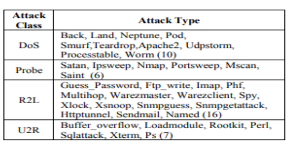
  2. Multinomial classification: Activity is normal or DOS or PROBE or R2L or U2R .

Data Availability:

This data is KDDCUP’99 data set, which is widely used as one of the few publicly available data sets for network-based anomaly detection systems.

For more about data you can visit to http://www.unb.ca/cic/datasets/nsl.html

BASIC FEATURES OF EACH NETWORK CONNECTION VECTOR

  1. Duration: Length of time duration of the connection
  2.  Protocol_type: Protocol used in the connection
  3.  Service: Destination network service used
  4.  Flag: Status of the connection – Normal or Error
  5.  Src_bytes: Number of data bytes transferred from source to destination in single connection
  6.  Dst_bytes: Number of data bytes transferred from destination to source in single connection
  7.  Land: if source and destination IP addresses and port numbers are equal then, this variable takes value 1 else 0
  8.  Wrong_fragment: Total number of wrong fragments in this connection
  9.  Urgent: Number of urgent packets in this connection. Urgent packets are packets with the urgent bit activated.
  10. Hot: Number of „hot‟ indicators in the content such as: entering a system directory, creating programs and executing programs.
  11. Num_failed _logins: Count of failed login attempts.
  12. Logged_in Login Status: 1 if successfully logged in; 0 otherwise.
  13. Num_compromised: Number of “compromised’ ‘ conditions.
  14. Root_shell: 1 if root shell is obtained; 0 otherwise.
  15.  Su_attempted: 1 if “su root” command attempted or used; 0 otherwise.
  16.  Num_root: Number of “root” accesses or number of operations performed as a root in the connection.
  17. Num_file_creations: Number of file creation operations in the connection.
  18. Num_shells: Number of shell prompts.
  19. Num_access_files: Number of operations on access control files .
  20. Num_outbound_cmds: Number of outbound commands in an ftp session.
  21. Is_hot_login: 1 if the login belongs to the “hot” list i.e., root or admin; else 0.
  22. Is_guest_login: 1 if the login is a “guest” login; 0 otherwise .
  23. Count: Number of connections to the same destination host as the current connection in the past two seconds
  24. Srv_count: Number of connections to the same service (port number) as the current connection in the past two seconds.
  25. Serror_rate: The percentage of connections that have activated the flag (4) s0, s1, s2 or s3, among the connections aggregated in count (23 )
  26. Srv_serror_rate: The percentage of connections that have activated the flag (4) s0, s1, s2 or s3, among the connections aggregated in srv_count (24)
  27. Rerror_rate: The percentage of connections that have activated the flag (4) REJ, among the connections aggregated in count (23)
  28. Srv_rerror_rate: The percentage of connections that have activated the flag (4) REJ, among the connections aggregated in srv_count (24)
  29. Same_srv_rate: The percentage of connections that were to the same service, among the connections aggregated in count (23)
  30. Diff_srv_rate: The percentage of connections that were to different services, among the connections aggregated in count (23)
  31. Srv_diff_host_ rate: The percentage of connections that were to different destination machines among the connections aggregated in srv_count (24)
  32. Dst_host_count: Number of connections having the same destination host IP address.
  33. Dst_host_srv_ count: Number of connections having the same port number.
  34. Dst_host_same _srv_rate: The percentage of connections that were to the same service, among the connections aggregated in dst_host_count (32) .
  35. Dst_host_diff_ srv_rate: The percentage of connections that were to different services, among the connections aggregated in dst_host_count (32)
  36. Dst_host_same _src_port_rate: The percentage of connections that were to the same source port, among the connections aggregated in dst_host_srv_c ount (33) .
  37. Dst_host_srv_ diff_host_rate: The percentage of connections that were to different destination machines, among the connections aggregated in dst_host_srv_count (33).
  38. Dst_host_serro r_rate: The percentage of connections that have activated the flag (4) s0, s1, s2 or s3, among the connections aggregated in dst_host_count (32).
  39. Dst_host_srv_s error_rate: The percent of connections that have activated the flag (4) s0, s1, s2 or s3, among the connections aggregated in dst_host_srv_c ount (33).
  40. Dst_host_rerro r_rate: The percentage of connections that have activated the flag (4) REJ, among the connections aggregated in dst_host_count (32) .
  41. Dst_host_srv_r error_rate: The percentage of connections that have activated the flag (4) REJ, among the connections aggregated in dst_host_srv_c ount (33).

Attack Class:

Let’s develop a machine learning model for further analysis.

Online Job Posting Analysis

Business Context:

The project seeks to understand the overall demand for labour in the Armenian online job market from the 19,000 job postings from 2004 to 2015 posted on Career Center, an Armenian human resource portal. Through text mining on this data, we will be able to understand the nature of the ever-changing job market, as well as the overall demand for labour in the Armenia economy. The data was originally scraped from a Yahoo! Mailing group.

Business Objectives:

Our main business objectives are to understand the dynamics of the labour market of Armenia using the online job portal post as a proxy. A secondary objective is to implement advanced text analytics as a proof of concept to create additional features such as enhanced search function that can add additional value to the users of the job portal.

So as a Data scientist you need to answer following business questions .

Job Nature and Company Profiles:

What are the types of jobs that are in demand in Armenia? How are the job natures changing over time?

Desired Characteristics and Skill-Sets:

What are the desired characteristics and skill -set of the candidates based on the job description dataset? How these are desired characteristics changing over time?

IT Job Classification:

Build a classifier that can tell us from the job description and company description whether a job is IT or not, so that this column can be automatically populated for new job postings. After doing so, understand what important factors are which drives this classification.

Similarity of Jobs:

Given a job title, find the 5 top jobs that are of a similar nature, based on the job post.

What should be our Text mining goal?

For the IT Job classification business question, you should aim to create supervised learning classification models that are able to classify based on the job text data accurately, is it an IT job.

On the business question of Job Nature and Company Profiles. Unsupervised learning techniques, such as topic modelling and other techniques such as term frequency counting will be applied to the data, including time period segmented dataset. Qualitative assessment will be done on the results to help us understand the job postings.

To understand the desired characteristics and skill -sets demanded by employers in the job ads, unsupervised learning methods such as K-means clustering will be used after appropriate dimension reduction.

For Job Queries business question, we propose exploring the usage of Latent Semantic Model and Matrix Similarity methods for information retrieval. The results will be assessed qualitatively. To return the top 5 most similar job posting, the job text data are vectorised using different models such as word2vec, and doc2vec and similarity scores are obtained using cosine similarity scores, ranked and returned as the answer which is then evaluated individually for relevance.

Data Understanding:

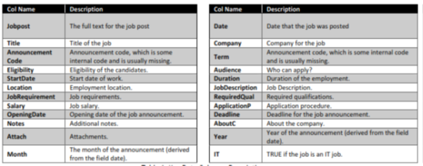
The data was obtained from Kaggle competition. Each row represents a job post. The dataset representation is tabular, but many of the columns are textual/unstructured in nature. Most notably, the columns job Description, Job Requirement, Required Qual, ApplicationP and AboutC are textual. The column job post is an amalgamation of these various textual columns.

Also provided sample job posting (attached with data set)

Let’s develop a machine learning model for further analysis.

PCA with python

In this lecture we will implement PCA algorithm through Python. We will also see how to reduce features in the data set.

About Minist Data Set

The MNIST dataset (Modified National Institute of Standards and Technology database) is a large dataset of handwritten digits that is commonly used for training various image processing systems. Available on kaggle (https://www.kaggle.com/c/digit-recognizer/data)

The database is also widely used for training and testing in the field of machine learning.

  • The dataset consists of pair, “handwritten digit image” and “label”. Digit ranges from 0 to 9, meaning 10 patterns in total. handwritten digit image: This is gray scale image with size 28 x 28 pixel.
  • label : This is actual digit number this handwritten digit image represents. It is either 0 to 9.

Our Objective

In this data sets around 42000 rows and 784 columns are available, we will try to reduce features from 784, so that we will have less features and maximum information.

Let’s explore the concept through jupyter notebook.

Linear Regression-Theory

Linear regression is a supervised machine learning technique where we need to predict a continuous output, which has a constant slope.

There are two main types of linear regression:

1. Simple Regression:

Through simple linear regression we predict response using single features.

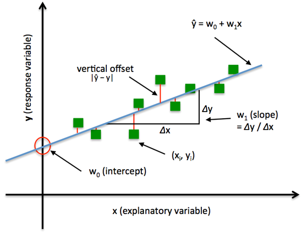
If you recall, the line equation (y = mx + c) we studied in schools. Let’s understand what these parameters say and how this equation works in linear regression.

Y = βo + β1X + ∈

Where, Y = Dependent Variable ( This is the variable which we want to predict )

            X = Independent Variable ( This is the variable which we use to make prediction )

            βo – This is the intercept term. It is the prediction value you get when X = 0

            β1 – This is the slope term. It explains the change in Y when X changes by 1 unit.

∈ – This represents the residual value, i.e. the difference between actual and predicted values.

2. Multivariable regression:

It is nothing but extension of simple linear regression. It attempts to model the relationship between two or more features and a response by fitting a linear equation to observed data.

Multi variable linear equation might look like this, where w represents the coefficients, or weights, our model will try to learn.

f(x,y,z)=w1x+w2y+w3z

Let’s understand it with example.

In a company for sales predictions, these attributes might include a company’s advertising spend on radio, TV, and newspapers.

Sales=w1Radio+w2TV+w3News

Linear Regression geometrical representation

So our goal in linear regression model is:

Find a line or plane that best fits the data points. Here best fit means minimise the sum of errors across our training data.

Types of Deliverable in linear regression:

Typically there are following questions that a business wanted to know

  1. They wanted to know their sales or profit prediction.
  2. Drivers(What drives the sales?)
    • All variable that have significant beta.
    • Which factors are detrimental /incremental?
    •  All the drivers, which one should target first?(Variable with highest absolute value)
  3. How to predict drivers?
    • To answer this question, you need calculate (beta*X )for each X variable and you need to choose the highest value and accordingly you can choose your driver after that convince business why you have chosen the particular driver.

So now the question arises how we calculate Beta values?

To calculate the beta values we will use OLS(ordinary least squared) method.

Assumptions of Linear Regression:

1. X variables (Explanatory variable) should be linearly related to Y (Response Variable):

Meaning:

If you plot a scatter plot between x variable and Y, most of the data point should be around the straight line.

How to check?

Draw the scatter plot between each x variable and y variable.

What happens if the assumption is violated?

MSE(Mean Squared Error) will be high. MSE is nothing but the average of squared error occurred between the predicted values and actual values. It can be written as:

Linear Regression in Machine Learning

Where,

N=Total number of observation
Yi = Actual value
(a1xi+a0)= Predicted value.

What to do if variable is not linear?

  • Drop the variable – But in this case will loose the information.
  • Take log(x+1) of x variables. 

2.Residual or the Y variable should be normally distributed:

Meaning:

Residuals (errors) or Y, when plotted in a histogram produces a bell shaped curve.

Residuals: The distance between the actual value and predicted values is called residual. If the observed points are far from the regression line, then the residual will be high, and so cost function will high. If the scatter points are close to the regression line, then the residual will be small and hence the cost function.

How to check?

Plot a histogram of Y, when plotted histogram produces a bell- shaped curve then it follows normality.

Or we can also use  q-q plot(quantile- quantile plot) of residuals

What happens if the assumption is violated?

It means all the P values has been calculated wrongly.

What to do if assumption is violated?

In that case we need to transform our Y such a way so that it become normal. To do that we need to use log of Y.

3.There should not be any relationship between X variables (i.e no multicollinearity)

Meaning:

X variable should not have any linear relationship between themselves. It’s obvious that we don’t want same information in repeat mode.

How to check?

  1. Calculate correlation between every X with every other X variable.
  2. Second method is to, calculate VIF(Variance influence factor)

What happens if the assumption is violated?

Your beta’s values sign will fluctuate.

What to do if assumption is violated?

Drop those X variable whose VIF is greater than 10(VIF>10)

4. The variance of error should remain constant over value of Y (Homoscedasticity/ No heteroskedasticity )

Meaning:

Spread of residuals should remain constant with values of Y.

How to check?

Draw scatter plot of residuals VS Y.

What happens if the assumption is violated?

Your P value will not accurate.

What to do if assumption is violated?

In that case we need to transform our Y such a way so that it become normal. To do that we need to use log of Y.

5. There should not be any auto-correlation between the residuals.

Meaning:

Correlation of residuals with lead residuals. Here lead residuals means next calculated residual.

How to check?

Use DW stats(Durbin Watson Stats)

            If DW stats ~ 2, then no auto correlation.

What happens if the assumption is violated?

Your P value will not accurate.

What to do if assumption is violated?

Understand the reason why it is happening?

If autocorrelation is due to Y then cannot build linear regression model.

If autocorrelation is due to X then drop that X variable.

How to check Model Performance?

The Goodness of fit determines how the line of regression fits the set of observations. The process of finding the best model out of various models is called optimization. It can be achieved by below method:

R-squared method:

  • R-squared is a statistical method that determines the goodness of fit.
  • It measures the strength of the relationship between the dependent and independent variables on a scale of 0-100%.
  • The high value of R-square determines the less difference between the predicted values and actual values and hence represents a good model.
  • It is also called a coefficient of determination, or coefficient of multiple determination for multiple regression.
  • It can be calculated from the below formula:
Linear Regression in Machine Learning

In the next lecture we will see how to implement leaner regression in python.

Linear regression with python

Company Objective:

Let’s suppose You just got some contract work with an Ecommerce company based in New York City that sells clothing online but they also have in-store style and clothing advice sessions. Customers come in to the store, have sessions/meetings with a personal stylist, then they can go home and order either on a mobile app or website for the clothes they want.

The company is trying to decide whether to focus their efforts on their mobile app experience or their website. They’ve hired you on contract to help them figure it out! Let’s get started!

Just follow the steps below to analyze the customer data (it’s fake, don’t worry I didn’t give you real credit card numbers or emails ). Click here to download

Click here to download .ipnyb notebook

Logistic Regression-Theory

As these days in analytics interview most of the interviewer ask questions about two algorithms which is logistic and linear regression. But why is there any reason behind?

Yes, there is a reason behind that these algorithm are very easy to interpret. I believe you should have in-depth understanding of these algorithms.

In this article we will learn about logistic regression in details. So let’s deep dive in Logistic regression.

What is Logistic Regression?

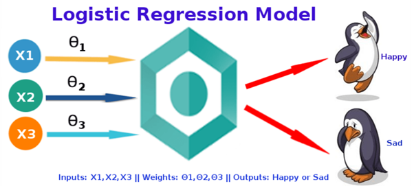
Logistic regression is a classification technique which helps to predict the probability of an outcome that can only have two values. Logistic Regression is used when the dependent variable (target) is categorical.

Types of logistic Regression:

  • Binary(Pass/fail or 0/1)
  • Multi(Cats, Dog, Sheep)
  • Ordinal(Low, Medium, High)

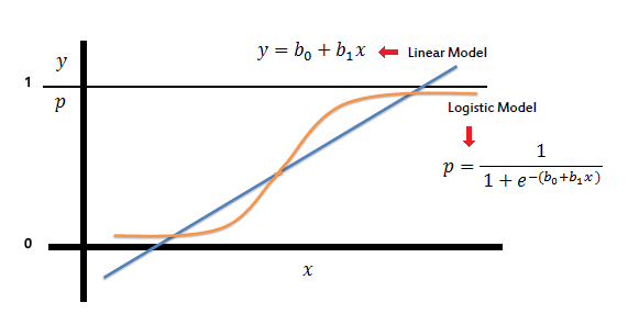
On the other hand, a logistic regression produces a logistic curve, which is limited to values between 0 and 1. Logistic regression is similar to a linear regression, but the curve is constructed using the natural logarithm of the “odds” of the target variable, rather than the probability.

What is Sigmoid Function:

To map predicted values with probabilities, we use the sigmoid function. The function maps any real value into another value between 0 and 1. In machine learning, we use sigmoid to map predictions to probabilities.

S(z) = 1/1+e−z

Where:

  • s(z)  = output between 0 and 1 (probability estimate)
  • z = input to the function (your algorithm’s prediction e.g.  b0 + b1*x)
  • e = base of natural log

Graph

In Linear Regression, we use the Ordinary Least Square (OLS) method to determine the best coefficients to attain good model fit but In Logistic Regression, we use maximum likelihood method to determine the best coefficients and eventually a good model fit.

How Maximum Likelihood method works?

For a binary classification (1/0), maximum likelihood will try to find the values of  b0 and b1 such that the resultant probabilities are close to either 1 or 0.

Logistic Regression Assumption:

I got a very good consolidated assumption on Towards Data science website, which I am putting here.

  • Binary logistic regression requires the dependent variable to be binary.
  • For a binary regression, the factor level 1 of the dependent variable should represent the desired outcome.
  • Only meaningful variables should be included.
  • The independent variables should be independent of each other. That is, the model should have little or no multicollinearity.
  • The independent variables are linearly related to the log of odds.
  • Logistic regression requires quite large sample sizes.

Performance evaluation methods of Logistic Regression.

Akaike Information Criteria (AIC):

We can say AIC works as a counter part of adjusted R square in multiple regression. The thumb rules of AIC are Smaller the better. AIC penalizes increasing number of coefficients in the model. In other words, adding more variables to the model wouldn’t let AIC increase. It helps to avoid overfitting.

To measure AIC of a single mode will not fruitful. To use AIC correctly build 2-3 logistic model and compare their AIC. The model which will have lowest AIC will relatively batter.

Null Deviance and Residual Deviance:

  • Null deviance is calculated from the model with no features, i.e. only intercept. The null model predicts class via a constant probability.
  • Residual deviance is calculated from the model having all the features. In both null and residual lower the value batter the model is.

Confusion Matrix:

It is nothing but a tabular representation of Actual vs Predicted values. This helps us to find the accuracy of the model and avoid overfitting. This is how it looks like

So now we can calculate the accuracy.

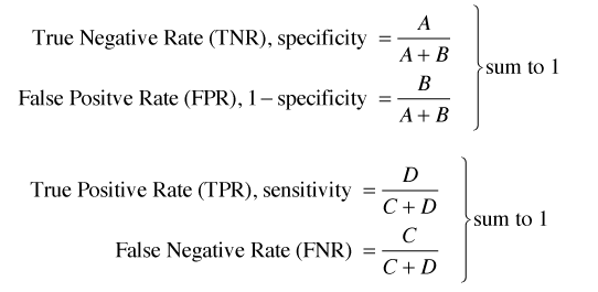
True Positive Rate (TPR):

It shows how many positive values, out of all the positive values, have been correctly predicted.

The formula to calculate the true positive rate is (TP/TP + FN). Or TPR =  1 - False Negative Rate. It is also known as Sensitivity or Recall.

False Positive Rate (FPR):

It shows how many negative values, out of all the negative values, have been incorrectly predicted.

The formula to calculate the false positive rate is (FP/FP + TN). Also, FPR = 1 - True Negative Rate.

True Negative Rate (TNR):

It represents how many negative values, out of all the negative values, have been correctly predicted. The formula to calculate the true negative rate is (TN/TN + FP). It is also known as Specificity.

False Negative Rate (FNR):

It indicates how many positive values, out of all the positive values, have been incorrectly predicted. The formula to calculate false negative rate is (FN/FN + TP).

Precision:

It indicates how many values, out of all the predicted positive values, are actually positive. The formula is (TP / TP + FP)

F Score:

F score is the harmonic mean of precision and recall. It lies between 0 and 1. Higher the value, better the model. Formula is  2((precision*recall) / (precision + recall)).

Receiver Operator Characteristic (ROC):

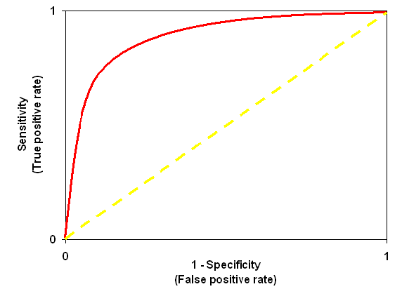
ROC is use to determine the accuracy of a classification model. It determines the model’s accuracy using Area Under Curve (AUC). Higher the area batter the model. ROC is plotted between True Positive Rate (Y axis) and False Positive Rate (X Axis).

In below graph yellow line represents the ROC curve at 0.5 thresholds. At this point, sensitivity = specificity.