Logistic regression to predict absenteeism- approach

Business Problem:

In today environment there is a high competitiveness which increase pressure on employee. High competitiveness leads unachievable goals, which cause an employee health issues, and health issue will lead absenteeism of employee.

With a given dataset an organisation is trying to predict employee absenteeism.

What is absenteeism in the business context?

Absence from work during normal working hours, resulting in temporary incapacity to execute regular working activity.

Purpose Of Model:

Explore whether a person presenting certain characteristics is expected to be away from work at some points in time or not.

Dataset:

I have downloaded a data set from kaggle called ‘Absenteeism_data.csv’ which contain following information.

  • Reason_1 – A Type of Reason to be absent.
  • Reason_2 – A Type of Reason to be absent.
  • Reason_3 – A Type of Reason to be absent.
  • Reason_4 – A Type of Reason to be absent.
  • Month Value – Month in which employee has been absent.
  • Day of the Week – Days
  • Transportation Expense – Expense in dollar
  • Distance to Work – Distance of workplace in Km
  • Age – Age of employee
  • Daily Work Load Average – Average amount of time spent working per day shown in minutes.
  • Body Mass Index – Body Mass index of employee.
  • Education – Education category(1 – high school education, 2 – Graduate, 3 – Post graduate, 4 – A Master or Doctor )
  • Children – No of children an employee has
  • Pet – Whether employee has pet or not?
  • Absenteeism Time in Hours – How many hours an employee has been absent.

Following are the main action we will take in this project.

  1. Build the model in python
  2. Save the result in Mysql.
  3. Visualise the end result in Tableau

Python for model building:

We are going to take following steps to predict absenteeism:

Load the data

Import the ‘Absenteeism_data.csv’ with the help of pandas

Identify dependent Variable i.e. identify the Y:

We have to be categories and we must find a way to say if someone is ‘being absent too much’ or not. what we’ve decided to do is to take the median of the dataset as a cut-off line in this way the dataset will be balanced (there will be roughly equal number of 0s and 1s for the logistic regression) as balancing is a great problem for ML, this will work great for us alternatively, if we had more data, we could have found other ways to deal with the issue for instance, we could have assigned some arbitrary value as a cut-off line, instead of the median.

Note that what line does is to assign 1 to anyone who has been absent 4 hours or more (more than 3 hours) that is the equivalent of taking half a day off initial code from the lecture targets = np.where(data_preprocessed[‘Absenteeism Time in Hours’] > 3, 1, 0)

Choose Algorithm to develop model:

As our Y (dependent variable) is 1 or o i.e. absent or not absent so we are going to use Logistic regression for our analysis.

Select Input for the regression:

We have to select our all x variables i.e. all independent variable which we will use for regression analysis.

Data Pre-processing:

Remove or treat missing value

In our case there is no missing value so we don’t have to worry about missing value. Yes, there are some columns who is not adding any value in our analysis such as ID which is unique in every case so we will remove it.

Remove Outliers

In our case there are no outliers so we don’t have to worry. But in general if you have outlier you can take log of your x variable to remove outliers.

Standardize the data

standardization is one of the most common pre-processing tools since data of different magnitude (scale) can be biased towards high values, we want all inputs to be of similar magnitude this is a peculiarity of machine learning in general – most (but not all) algorithms do badly with unscaled data. A very useful module we can use is Standard Scaler. It has much more capabilities than the straightforward ‘pre-processing’ method. We will create a variable that will contain the scaling information for this particular dataset.

Here’s the full documentation:

http://scikitlearn.org/stable/modules/generated/sklearn.preprocessing.StandardScaler.html

Choose the column to scales

In this section we need to choose that variable which need to transform or scale.in our case we need to scale  [‘Reason_1’, ‘Reason_2’, ‘Reason_3’, ‘Reason_4′,’Education’, pet and ‘children’], because these are the columns  which contain categorical data but in numerical form so we need to transform them.

What about the other column?

‘Month Value’, ‘Day of the Week’,  ‘Transportation Expense’,  ‘Distance to Work’,  ‘Age’, ‘Daily Work Load Average’, ‘Body Mass Index’ . These are the numerical value and their data type is int. so we do not have to transform them but will keep in our analysis.

Note:-

You can ask why we are doing analysis manually column wise?

Because it is always good to analyse data feature wise it gives us a confidence for our model and we can easily interpret our model analysis.

Split Data into train and test

Divide our data into train and test and build the model on train data set.

Apply Algorithm

As per our scenario we are going to use logistic regression in our case. Following steps will take place

Train the model

First we will divide the data into train and test. We will build our model on train data set.

Test the model

When we successfully developed our model then we need to test with a new data set which is testing data sets.

Find the intercepts and coefficient

Find out the beta values and coefficient from model.

Interpreting the coefficients

Find out which feature is adding more values in predictions of Y.

Save the model

Need to save the model which we have prepared so far. To do that we need to pickle the model.

Two executable file will save in your python directory one ‘model’ and the other is ‘scaler’

To save your .Ipnyb file in form of executable, save the same as .py file.

Check Model performance on totally new data set with same features.

Now we have a totally new data set which has same feature as per previous data set but contain different values.

Note – To do that your executable file ‘model’, scaler’ and ‘.py’ file should be in same folder.

Mysql for Data store

Save the prediction in data base (Mysql)

It is always good to save data and prediction on centralised data base.  So create a data base in mysql and create a table with all field available in your predicted data frame i.e ‘df_new_obs’

Import ‘pymysql’ library to make connection between ipynb notebook and mysql.

Setup the connection with user name and password and insert the predicted output values. In the data base.

Tableau for Data visualization

Connect the data base with Tableau and visualize the result

As we know tableau is a strong tool to visualise the data. So in our case we will connect our database with tableau and visualise our result and present to the business.

To connect tableau with my sql we need to take following steps.

  • Open the tableau desktop application.
  • Click on connect data source as mysql.
  • Put your data base address, username and password.
  • Select the data base.
  • Drag the table and visualize your data.

Network Intrusion Detection

In this case study we need to predict anomalies and attacks in the network.

Business Problem:

The task is to build network intrusion detection system to detect anomalies and attacks in the network.

There are two problems.

  1. Binomial Classification: Activity is normal or attack.
  2. Multinomial classification: Activity is normal or DOS or PROBE or R2L or U2R .

Data Availability:

This data is KDDCUP’99 data set, which is widely used as one of the few publicly available data sets for network-based anomaly detection systems.

For more about data you can visit to http://www.unb.ca/cic/datasets/nsl.html

BASIC FEATURES OF EACH NETWORK CONNECTION VECTOR

  1. Duration: Length of time duration of the connection
  2.  Protocol_type: Protocol used in the connection
  3.  Service: Destination network service used
  4.  Flag: Status of the connection – Normal or Error
  5.  Src_bytes: Number of data bytes transferred from source to destination in single connection
  6.  Dst_bytes: Number of data bytes transferred from destination to source in single connection
  7.  Land: if source and destination IP addresses and port numbers are equal then, this variable takes value 1 else 0
  8.  Wrong_fragment: Total number of wrong fragments in this connection
  9.  Urgent: Number of urgent packets in this connection. Urgent packets are packets with the urgent bit activated.
  10. Hot: Number of „hot‟ indicators in the content such as: entering a system directory, creating programs and executing programs.
  11. Num_failed _logins: Count of failed login attempts.
  12. Logged_in Login Status: 1 if successfully logged in; 0 otherwise.
  13. Num_compromised: Number of “compromised’ ‘ conditions.
  14. Root_shell: 1 if root shell is obtained; 0 otherwise.
  15.  Su_attempted: 1 if “su root” command attempted or used; 0 otherwise.
  16.  Num_root: Number of “root” accesses or number of operations performed as a root in the connection.
  17. Num_file_creations: Number of file creation operations in the connection.
  18. Num_shells: Number of shell prompts.
  19. Num_access_files: Number of operations on access control files .
  20. Num_outbound_cmds: Number of outbound commands in an ftp session.
  21. Is_hot_login: 1 if the login belongs to the “hot” list i.e., root or admin; else 0.
  22. Is_guest_login: 1 if the login is a “guest” login; 0 otherwise .
  23. Count: Number of connections to the same destination host as the current connection in the past two seconds
  24. Srv_count: Number of connections to the same service (port number) as the current connection in the past two seconds.
  25. Serror_rate: The percentage of connections that have activated the flag (4) s0, s1, s2 or s3, among the connections aggregated in count (23 )
  26. Srv_serror_rate: The percentage of connections that have activated the flag (4) s0, s1, s2 or s3, among the connections aggregated in srv_count (24)
  27. Rerror_rate: The percentage of connections that have activated the flag (4) REJ, among the connections aggregated in count (23)
  28. Srv_rerror_rate: The percentage of connections that have activated the flag (4) REJ, among the connections aggregated in srv_count (24)
  29. Same_srv_rate: The percentage of connections that were to the same service, among the connections aggregated in count (23)
  30. Diff_srv_rate: The percentage of connections that were to different services, among the connections aggregated in count (23)
  31. Srv_diff_host_ rate: The percentage of connections that were to different destination machines among the connections aggregated in srv_count (24)
  32. Dst_host_count: Number of connections having the same destination host IP address.
  33. Dst_host_srv_ count: Number of connections having the same port number.
  34. Dst_host_same _srv_rate: The percentage of connections that were to the same service, among the connections aggregated in dst_host_count (32) .
  35. Dst_host_diff_ srv_rate: The percentage of connections that were to different services, among the connections aggregated in dst_host_count (32)
  36. Dst_host_same _src_port_rate: The percentage of connections that were to the same source port, among the connections aggregated in dst_host_srv_c ount (33) .
  37. Dst_host_srv_ diff_host_rate: The percentage of connections that were to different destination machines, among the connections aggregated in dst_host_srv_count (33).
  38. Dst_host_serro r_rate: The percentage of connections that have activated the flag (4) s0, s1, s2 or s3, among the connections aggregated in dst_host_count (32).
  39. Dst_host_srv_s error_rate: The percent of connections that have activated the flag (4) s0, s1, s2 or s3, among the connections aggregated in dst_host_srv_c ount (33).
  40. Dst_host_rerro r_rate: The percentage of connections that have activated the flag (4) REJ, among the connections aggregated in dst_host_count (32) .
  41. Dst_host_srv_r error_rate: The percentage of connections that have activated the flag (4) REJ, among the connections aggregated in dst_host_srv_c ount (33).

Attack Class:

Let’s develop a machine learning model for further analysis.

Decision Tree – Theory

Decision tree is very simple yet a powerful algorithm for classification and regression. As name suggest it has tree like structure. It is a non-parametric technique. A decision tree typically starts with a single node, which branches into possible outcomes. Each of those outcomes leads to additional nodes, which branch off into other possibilities. This gives it a treelike shape.

For example of a decision tree can be explained using below binary tree. Let’s suppose you want to predict whether a person is fit by their given information like age, eating habit, and physical activity, etc. The decision nodes here are questions like ‘What’s the age?’, ‘Does he exercise?’, ‘Does he eat a lot of pizzas’? And the leaves, which are outcomes like either ‘fit’, or ‘unfit’. In this case this was a binary classification problem (yes or no type problem).

There are two main types of Decision Trees:

Classification trees (Yes/No types)

What we’ve seen above is an example of classification tree, where the outcome was a variable like ‘fit’ or ‘unfit’. Here the decision variable is categorical.

Regression trees (Continuous data types)

Here the decision or the outcome variable is Continuous, e.g. a number like 123.

Image source google.com

The top-most item, in this example, “Age < 30 ?” is called the root. It’s where everything starts from. Branches are what we call each line. A leaf is everything that isn’t the root or a branch.

A general algorithm for a decision tree can be described as follows:

  1. Pick the best attribute/feature. The best attribute is one which best splits or separates the data.
  2. Ask the relevant question.
  3. Follow the answer path.
  4. Go to step 1 until you arrive to the answer.

Terms used with Decision Trees:

  1. Root Node – It represents entire population or sample and this further gets divided into two or more similar sets.
  2. Splitting – Process to divide a node into two or more sub nodes.
  3. Decision Node – A sub node is divided further sub node, called decision node.
  4. Leaf/Terminal Node – Node which do not split further called leaf node.
  5. Pruning – When we remove sub-nodes of a decision node, this process is called pruning.
  6. Branch/ Sub-tree – A sub-section of entire tree is called branch or subtree.
  7. Parent and child node – A node, which is divided into sub-nodes is called parent node of sub-nodes whereas sub-nodes are the child of parent node.

Let’s understand above terms with the below image

Image Source google.com

Types of Decision Trees

  1. Categorical Variable decision tree – Decision Tree which has categorical target variable then it called as categorical variable.
  2. Continuous Variable Decision Tree – Decision Tree which has continuous target variable then it is called as Continuous Variable Decision Tree.

Advantages of Decision Tree

  1. Easy to understand – Algorithm is very easy to understand even for people from non-analytical background. A person without statistical knowledge can interpret them.
  2. Useful in data exploration – It is the fastest algorithm to identify most significant variables and relation between variables. It help us to identify those variables which has better power to predict target variable.
  3. Decision tree do not required more effort from user side for data preparation.
  4. This algorithm is not affected by outliers or missing value to an extent, so it required less data cleaning effort as compare to other model.
  5. This model can handle both numerical and categorical variables.
  6. The number of hyper-parameters to be tuned is almost null.

Disadvantages of Decision Tree

  1. Over Fitting – It is the most common problem in decision tree. This issue has resolved by setting constraints on model parameters and pruning. Over fitting is an phenomena where your model create a complex tree that do not generalize the data very well.
  2. Small variations in the data can result completely different tree which mean it unstable the model. This problem is called variance, which need to lower by method like bagging and boosting.
  3. If some class is dominate in your model then decision tree learner can create a biased tree. So it is recommended to balance the data set prior to fitting with the decision tree.
  4. Calculations can become complex when there are many class label.

Decision Tree Flowchart

Image Source google.com

How does a tree decide where to split?

In decision tree making splits effect the accuracy of model. The decision criteria are different for classification and regression trees. Decision tree splits the nodes on all available variables and then selects the split which results in most homogeneous sub-nodes.

The algorithm selection is also based on type of target variables. The four most commonly used algorithms in decision tree are:

  1. CHAID – Chi-Square Interaction Detector
  2. CART – Classification and regression trees.

Let’s discuss both methods in detail

CHAID – Chi-Square Interaction Detector

It is an algorithm to find out the statistical significance between the differences between sub-nodes and parent node. It works with categorical target variable such as “yes” or “no”.

Algorithm follows following steps:

  1. Iterate all available x variables.
    1. Check if the variable is numeric
    2. If the variable is numeric make it categorical by decile and percentile.
    3. Figure out all possible cuts.
    4. For each possible cut it will do Chi-Square test and store the P value
    5. Choose that cut which give least p value.
  2. Cut the data using that variable and that cut which gives least P value.

CART – Classification and regression trees

There are basically two subtypes for this algorithm.

Gini index:

It says, if we select two items from a population at random then they must be of same class and probability for this is 1 if population is pure. It works with categorical target variable “Success” or “Failure”.

Gini = 1-P^2 – (1-p)^2 , Here p is the probability

Gain = Gini of parents leaf – weighted average of Gini of the nodes (Weights are proportional to population of each child node)

Steps to Calculate Gini for a split

  1. Iterate all available x variables.
    1. Check if the variable is numeric
    2. If the variable is numeric make it categorical by decile and percentile.
    3. Figure out all possible cuts.
    4. Calculate gain for each split
    5. Choose that cut which gives the highest cut.
  2. Cut the data using that variable and that cut which gives maximum gain

Entropy Tree:

To understand entropy tree we need to first understand what entropy is?

Entropy – Entropy is basically measures the level of impurity in a group of examples. If the sample is completely homogeneous, then the entropy is zero and if the sample is an equally divided (50% — 50%), it has entropy of one.

Entropy = -p log2 p — q log2q

Here p and q is the probability of success and failure respectively in that node. Entropy is also used with categorical target variable. It chooses the split which has lowest entropy compared to parent node and other splits. The lesser the entropy, the better it is.

Gain = Entropy of parents leaf – weighted average of entropy of the nodes (Weights are proportional to population of each child node)

Steps to Calculate Entropy for a split

  1. Iterate all available x variables.
    1. Check if the variable is numeric
    2. If the variable is numeric make it categorical by decile and percentile.
    3. Figure out all possible cuts.
    4. Calculate gain for each split
    5. Choose that cut which gives the highest cut.
  2. Cut the data using that variable and that cut which gives maximum gain.

Decision Tree Regression

As we have discussed above with the help of decision tree we can also solve the regression problem. So let’s see what the steps are.

Following steps are involved in algorithm.

  1. Iterate all available x variables.
    1. Check if the variable is numeric
    2. If the variable is numeric make it categorical by decile and percentile.
    3. Figure out all possible cuts.
    4. For each cuts calculate MSE
    5. Choose that cut and that variable which gives the minimum MSE.
  2. Cut the data using that variable and that cut which gives minimum MSE.

Stopping Criteria of Decision Tree

  1. Pure Node – If tree find a pure node, that particular leaf will stop growing.
  2. User defined depth
  3. Minimum observation in the node
  4. Minimum observation in the leaf

Bagging & Boosting – Theory

Bagging

Bootstrap Aggregation (or Bagging for short), is a simple and very powerful ensemble method. Bootstrap method refers to random sampling with replacement. Here with replacement means a sample can be repetitive. Bagging allows model or algorithm to get understand about various biases and variance.

To create bagging model, first we create multiple random samples so that each new random sample will act as another (almost) independent dataset drawn from original distribution. Then, we can fit a weak learner for each of these samples and finally aggregate their outputs and obtain an ensemble model with less variance from its components.

Let’s understand it with an eg.as we can see in below figure where each sample population has different pieces and none of them are identical. This would then affect the overall mean, standard deviation and other descriptive metrics of a data set.  It develops more robust models.

How bagging works

How Bagging Works?

  1. You generate multiple samples from your training set using next scheme: you take randomly an element from training set and then return it back. So, some of elements of training set will present multiple times in generated sample and some will be absent. These samples should have the same size as the train set.
  2. You train you learner on each generated sample.
  3. When you apply the algorithm you just average predictions of learners in case of regression or make the voting in case of classification.

Applying bagging often help to deal with overfitting by reducing prediction variance.

Bagging Algorithms:

  1. Take M bootstrap samples (with replacement)
  2. Train M different classifiers on these bootstrap samples
  3. For a new query, let all classifiers predict and take an average(or majority vote)
  4. If the classifiers make independent errors, then their ensembles can improve performance.

Boosting:

Boosting is an ensemble modeling technique which converts weak learner to strong learners.

Let’s understand it with an example. Let’s suppose you want to identify an email is a SPAM or NOT SPAM. To do that you need to take some criteria as follows.

  1. Email has only one image file, It’s a SPAM
  2. Email has only link, It’s a SPAM
  3. Email body consist of sentence like “You won a prize money of $ xxxx”, It’s a SPAM
  4. Email from our official domain “datasciencelovers.com”, Not a SPAM
  5. Email from known source, Not a SPAM

As we can see above there are multiple rules to identify an email is a spam or not. But if we will talk about individual rules they are not as powerful as multiple rules. There these individual rules is a weak learner.

To convert weak learner to strong learner, we’ll combine the prediction of each weak learner using methods like:
•   Using average/ weighted average
•   Considering prediction has higher vote

For example:  Above, we have defined 5 weak learners. Out of these 5, 3 are voted as ‘SPAM’ and 2 are voted as ‘Not a SPAM’. In this case, by default, we’ll consider an email as SPAM because we have higher (3) vote for ‘SPAM’

Boosting Algorithm:

  1. The base learner takes all the distributions and assigns equal weight or attention to each observation.
  2. If there is any prediction error caused by first base learning algorithm, then we pay higher attention to observations having prediction error. Then, we apply the next base learning algorithm.
  3. Iterate Step 2 till the limit of base learning algorithm is reached or higher accuracy is achieved.

Finally, it combines the outputs from weak learner and creates a strong learner which eventually improves the prediction power of the model.

Types of Boosting Algorithm:

  1. AdaBoost (Adaptive Boosting)
  2. Gradient Tree Boosting
  3. XGBoost

AdaBoost(Adaptive Boosting)

Adaboost was the first successful and very popular boosting algorithm which developed for the purpose of binary classification. AdaBoost technique which combines multiple “weak classifiers” into a single “strong classifier”.

  1. Initialise the dataset and assign equal weight to each of the data point.
  2. Provide this as input to the model and identify the wrongly classified data points
  3. Increase the weight of the wrongly classified data points.
  4. if (got required results)
      Go to step 5
    else
      Go to step 2
  5. End

Let’s understand the concept with following example.

BOX – 1: In box 1 we have assigned equal weight to each data points and applied a decision stump to classify them as  + (plus) or – (minus). The decision stump (D1) has generated vertical line at left side to classify the data points. As we can see in the box vertical line has incorrectly predicted three + (plus) as – (minus). In this case, we will assign higher weights to these three + (plus) and apply another decision stump. As you can see in below image.

Decision stump – 1

BOX – 2: Now in box 2 size of three incorrectly predicted + (plus) is bigger as compared to rest of the data points. In this case, the second decision stump (D2) will try to predict them correctly. Now, a vertical line (D2) at right side of this box has classified three mis-classified + (plus) correctly. But in this process, it has caused mis-classification errors again. This time with three -(minus). So we will assign higher weight to three – (minus) and apply another decision stump. As you can see in below image.

Decision stump -2

BOX – 3: In box 3 there are three – (minus) has been given higher weights. A decision stump (D3) is applied to predict these mis-classified observation correctly. This time a horizontal line is generated to classify + (plus) and – (minus) based on higher weight of mis-classified observation.

Decision stump – 3

BOX – 4: in box 4 we will combine D1, D2 and D3 to form a strong prediction having complex rule as compared to individual weak learner. As we can see this algorithm has classified these observation quite well as compared to any of individual weak learner.

Decision Stump – 4

Python Code

from sklearn.ensamble import AdaBoostClassifier
clf = AdaBoostClassifier(n_estimators=4, random_state=0, algorithm=’SAMME’)
clf.fit(X, Y)

  • n_estimators : integer, optional (default=50)

The maximum number of estimators at which boosting is terminated. In case of perfect fit, the learning procedure is stopped early.

  • random_state : int, RandomState instance or None, optional (default=None)
  • algorithm : {‘SAMME’, ‘SAMME.R’}, optional (default=’SAMME.R’)

If ‘SAMME.R’ then use the SAMME.R real boosting algorithm. base estimator must support calculation of class probabilities. If ‘SAMME’ then use the SAMME discrete boosting algorithm.