Tag algorithm

Company Objective:

Let’s suppose You just got some contract work with an Ecommerce company based in New York City that sells clothing online but they also have in-store style and clothing advice sessions. Customers come in to the store, have sessions/meetings with a personal stylist, then they can go home and order either on a mobile app or website for the clothes they want.

The company is trying to decide whether to focus their efforts on their mobile app experience or their website. They’ve hired you on contract to help them figure it out! Let’s get started!

Just follow the steps below to analyze the customer data (it’s fake, don’t worry I didn’t give you real credit card numbers or emails ). Click here to download

Click here to download .ipnyb notebook

As these days in analytics interview most of the interviewer ask questions about two algorithms which is logistic and linear regression. But why is there any reason behind?

Yes, there is a reason behind that these algorithm are very easy to interpret. I believe you should have in-depth understanding of these algorithms.

In this article we will learn about logistic regression in details. So let’s deep dive in Logistic regression.

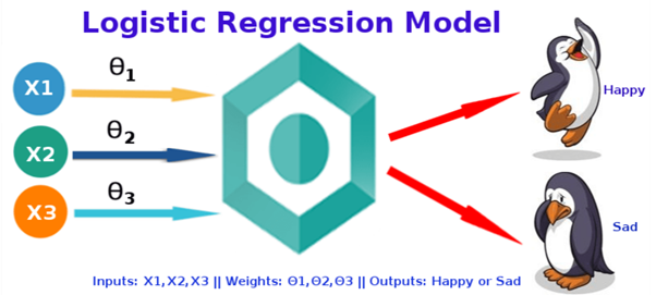
What is Logistic Regression?

Logistic regression is a classification technique which helps to predict the probability of an outcome that can only have two values. Logistic Regression is used when the dependent variable (target) is categorical.

Types of logistic Regression:

• Binary(Pass/fail or 0/1)
• Multi(Cats, Dog, Sheep)
• Ordinal(Low, Medium, High)

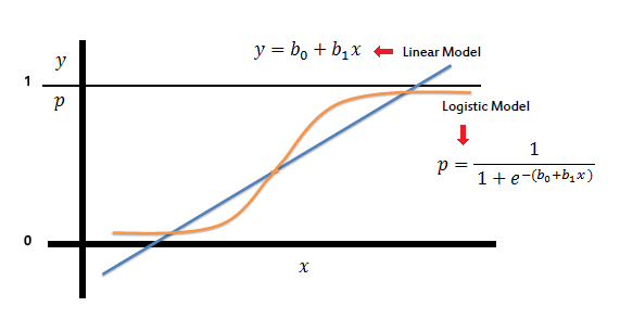
On the other hand, a logistic regression produces a logistic curve, which is limited to values between 0 and 1. Logistic regression is similar to a linear regression, but the curve is constructed using the natural logarithm of the “odds” of the target variable, rather than the probability.

What is Sigmoid Function:

To map predicted values with probabilities, we use the sigmoid function. The function maps any real value into another value between 0 and 1. In machine learning, we use sigmoid to map predictions to probabilities.

S(z) = 1/1+e−z

Where:

• s(z)  = output between 0 and 1 (probability estimate)
• z = input to the function (your algorithm’s prediction e.g.  b0 + b1*x)
• e = base of natural log

Graph

In Linear Regression, we use the Ordinary Least Square (OLS) method to determine the best coefficients to attain good model fit but In Logistic Regression, we use maximum likelihood method to determine the best coefficients and eventually a good model fit.

How Maximum Likelihood method works?

For a binary classification (1/0), maximum likelihood will try to find the values of  b0 and b1 such that the resultant probabilities are close to either 1 or 0.

Logistic Regression Assumption:

I got a very good consolidated assumption on Towards Data science website, which I am putting here.

• Binary logistic regression requires the dependent variable to be binary.
• For a binary regression, the factor level 1 of the dependent variable should represent the desired outcome.
• Only meaningful variables should be included.
• The independent variables should be independent of each other. That is, the model should have little or no multicollinearity.
• The independent variables are linearly related to the log of odds.
• Logistic regression requires quite large sample sizes.

Performance evaluation methods of Logistic Regression.

Akaike Information Criteria (AIC):

We can say AIC works as a counter part of adjusted R square in multiple regression. The thumb rules of AIC are Smaller the better. AIC penalizes increasing number of coefficients in the model. In other words, adding more variables to the model wouldn’t let AIC increase. It helps to avoid overfitting.

To measure AIC of a single mode will not fruitful. To use AIC correctly build 2-3 logistic model and compare their AIC. The model which will have lowest AIC will relatively batter.

Null Deviance and Residual Deviance:

• Null deviance is calculated from the model with no features, i.e. only intercept. The null model predicts class via a constant probability.

• Residual deviance is calculated from the model having all the features. In both null and residual lower the value batter the model is.

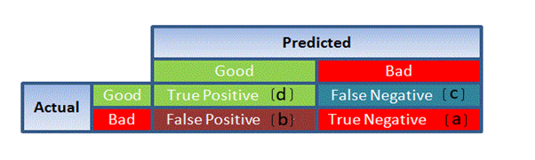
Confusion Matrix:

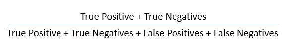
It is nothing but a tabular representation of Actual vs Predicted values. This helps us to find the accuracy of the model and avoid overfitting. This is how it looks like

So now we can calculate the accuracy.

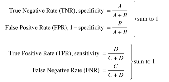
True Positive Rate (TPR):

It shows how many positive values, out of all the positive values, have been correctly predicted.

The formula to calculate the true positive rate is (TP/TP + FN). Or TPR =  1 - False Negative Rate. It is also known as Sensitivity or Recall.

False Positive Rate (FPR):

It shows how many negative values, out of all the negative values, have been incorrectly predicted.

The formula to calculate the false positive rate is (FP/FP + TN). Also, FPR = 1 - True Negative Rate.

True Negative Rate (TNR):

It represents how many negative values, out of all the negative values, have been correctly predicted. The formula to calculate the true negative rate is (TN/TN + FP). It is also known as Specificity.

False Negative Rate (FNR):

It indicates how many positive values, out of all the positive values, have been incorrectly predicted. The formula to calculate false negative rate is (FN/FN + TP).

Precision:

It indicates how many values, out of all the predicted positive values, are actually positive. The formula is (TP / TP + FP). 

F Score:

F score is the harmonic mean of precision and recall. It lies between 0 and 1. Higher the value, better the model. Formula is  2((precision*recall) / (precision + recall)).

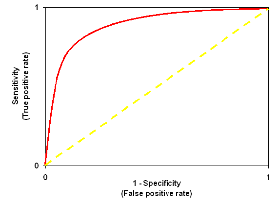
Receiver Operator Characteristic (ROC):

ROC is use to determine the accuracy of a classification model. It determines the model’s accuracy using Area Under Curve (AUC). Higher the area batter the model. ROC is plotted between True Positive Rate (Y axis) and False Positive Rate (X Axis).

In below graph yellow line represents the ROC curve at 0.5 thresholds. At this point, sensitivity = specificity.

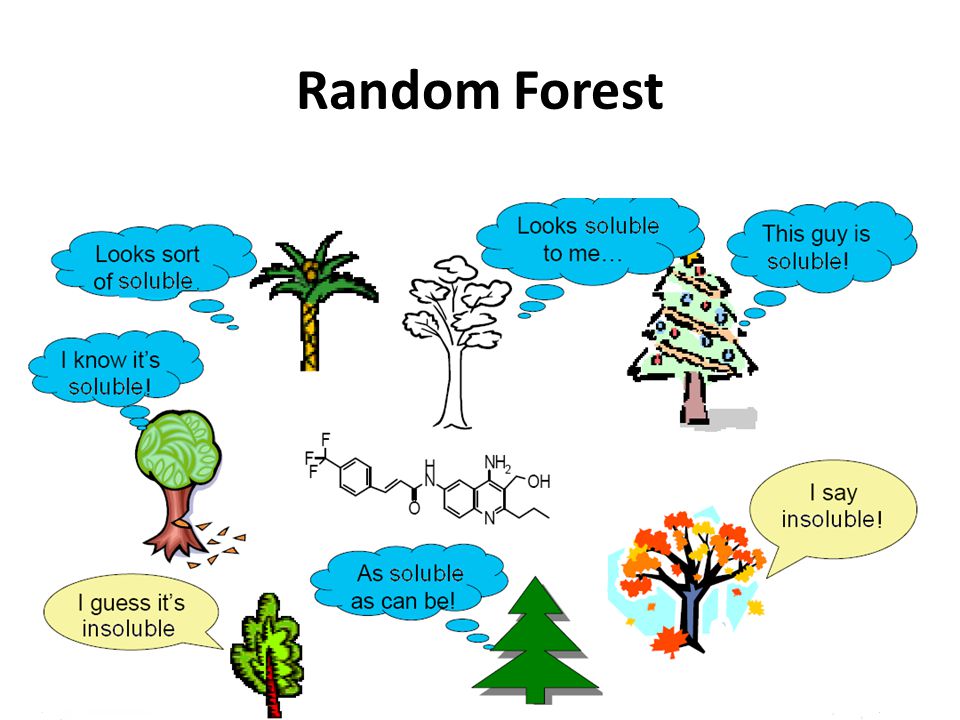
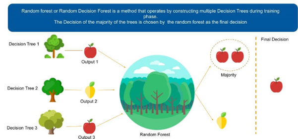
Random forest algorithm is a supervised algorithm. As you can guess from its name this algorithm creates a forest with number of trees. It operates by constructing multiple decision trees. The final decision is made based on the majority of the trees and is chosen by the random forest.

The method of combining trees is known as an ensemble method. Ensembling is nothing but a combination of weak learners (individual trees) to produce a strong learner.

Let’s understand ensemble with an example. Let’s suppose you want to watch movie but you have doubt in your mind regarding it’s reviews, so you have asked 10 people who have watched the movie, 8 of them said movie is fantastic and 2 of them said movie was not good. Since the majority is in favour, you decide to watch the movie. This is how we use ensemble techniques in our daily life too.

Random Forest can be used to solve regression and classification problems. In regression problems, the dependent variable is continuous. In classification problems, the dependent variable is categorical.

Advantages and Disadvantages of Random Forest

Advantages are as follows:

1. It is used to solve both regression and classification problems.
2. It can be also used to solve unsupervised ML problems.
3. It can handle thousands of input variables without variable selection.
4. It can be used as a feature selection tool using its variable importance plot.
5. It takes care of missing data internally in an effective manner.

Disadvantages are as follows:

1. This is a black-box model so Random Forest model is difficult to interpret.
2. It can take longer than expected time to computer a large number of trees.

How Random Forest works?

Algorithm can be divided into two stages.

• Random forest creation.
• Perform prediction from the created random forest classifier.

Random forest creation:

To create random forest we need to select following steps

1. Randomly select “k” features from total “m” features, where k << m.
2. Among the “k” features, calculate the node “d” using the best split point.
3. Split the node into child nodes using the best split.
4. Repeat 1 to 3 steps until “L” number of nodes has been reached.
5. Build forest by repeating steps 1 to 4 for “n” number times to create “n” number of trees.

Perform prediction from the created random forest classifier

To perform prediction we need to take following steps

1. Takes the test features and use the rules of each randomly created decision tree to predict the outcomes and stores the predicted outcome (target)
2. Calculate the votes for each predicted target.
3. Consider the high voted predicted target as the final prediction from the random forest algorithm.

Set the parameters for the random forest model:

Parameters = {‘bootstrap’: True,’min_samples_leaf’: 3, ‘n_estimators’: 50, ‘min_samples_split’: 10, ‘max_features’: ‘sqrt’,’max_depth’: 6,’max_leaf_nodes’: None} 

Hyperparameters Tuning of Random forest classifier:

bootstrap : boolean, optional (default=True)

min_samples_leaf : int, float, optional (default=1)

The minimum number of samples required to be at a leaf node:

• If int, then consider min_samples_leaf as the minimum number.
• If float, then min_samples_leaf is a percentage and ceil(min_samples_leaf * n_samples) are the minimum number of samples for each node.

n_estimators : integer, optional (default=10):

• The number of trees in the forest.

min_samples_split : int, float, optional (default=2):

The minimum number of samples required to split an internal node:

• If int, then consider min_samples_split as the minimum number.
• If float, then min_samples_split is a percentage and ceil(min_samples_split * n_samples) are the minimum number of samples for each split.

max_features : int, float, string or None, optional (default=”auto”):

The number of features to consider when looking for the best split:

• If int, then consider max_features features at each split. -If float, then max_features is a percentage and int(max_features * n_features) features are considered at each split.
• If “auto”, then max_features=sqrt(n_features).
• If “sqrt”, then max_features=sqrt(n_features) (same as “auto”).
• If “log2”, then max_features=log2(n_features).
• If None, then max_features=n_features.

max_depth : integer or None, optional (default=None):

The maximum depth of the tree. If None, then nodes are expanded until all leaves are pure or until all leaves contain less than min_samples_split samples.

max_leaf_nodes : int or None, optional (default=None):

Grow trees with max_leaf_nodes in best-first fashion. Best nodes are defined as relative reduction in impurity. If None then unlimited number of leaf nodes.

If you want to learn more about the rest of hyperparameters , check here

Bagging

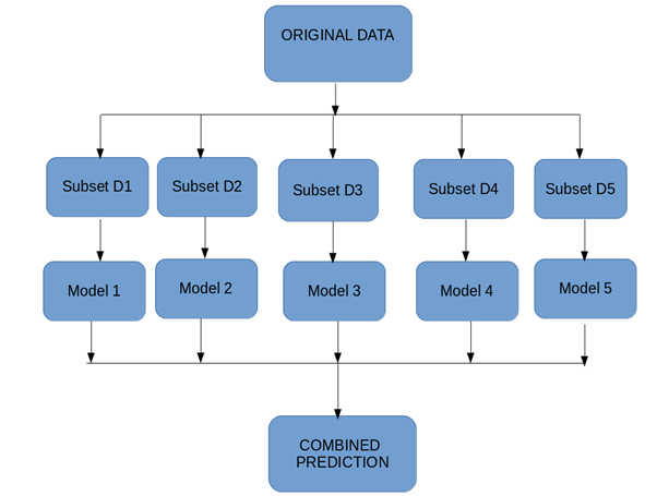
Bootstrap Aggregation (or Bagging for short), is a simple and very powerful ensemble method. Bootstrap method refers to random sampling with replacement. Here with replacement means a sample can be repetitive. Bagging allows model or algorithm to get understand about various biases and variance.

To create bagging model, first we create multiple random samples so that each new random sample will act as another (almost) independent dataset drawn from original distribution. Then, we can fit a weak learner for each of these samples and finally aggregate their outputs and obtain an ensemble model with less variance from its components.

Let’s understand it with an eg.as we can see in below figure where each sample population has different pieces and none of them are identical. This would then affect the overall mean, standard deviation and other descriptive metrics of a data set.  It develops more robust models.

How Bagging Works?

1. You generate multiple samples from your training set using next scheme: you take randomly an element from training set and then return it back. So, some of elements of training set will present multiple times in generated sample and some will be absent. These samples should have the same size as the train set.
2. You train you learner on each generated sample.
3. When you apply the algorithm you just average predictions of learners in case of regression or make the voting in case of classification.

Applying bagging often help to deal with overfitting by reducing prediction variance.

Bagging Algorithms:

1. Take M bootstrap samples (with replacement)
2. Train M different classifiers on these bootstrap samples
3. For a new query, let all classifiers predict and take an average(or majority vote)
4. If the classifiers make independent errors, then their ensembles can improve performance.

Boosting:

Boosting is an ensemble modeling technique which converts weak learner to strong learners.

Let’s understand it with an example. Let’s suppose you want to identify an email is a SPAM or NOT SPAM. To do that you need to take some criteria as follows.

1. Email has only one image file, It’s a SPAM
2. Email has only link, It’s a SPAM
3. Email body consist of sentence like “You won a prize money of $ xxxx”, It’s a SPAM
4. Email from our official domain “datasciencelovers.com”, Not a SPAM
5. Email from known source, Not a SPAM

As we can see above there are multiple rules to identify an email is a spam or not. But if we will talk about individual rules they are not as powerful as multiple rules. There these individual rules is a weak learner.

To convert weak learner to strong learner, we’ll combine the prediction of each weak learner using methods like:
•   Using average/ weighted average
•   Considering prediction has higher vote

For example:  Above, we have defined 5 weak learners. Out of these 5, 3 are voted as ‘SPAM’ and 2 are voted as ‘Not a SPAM’. In this case, by default, we’ll consider an email as SPAM because we have higher (3) vote for ‘SPAM’

Boosting Algorithm:

1. The base learner takes all the distributions and assigns equal weight or attention to each observation.
2. If there is any prediction error caused by first base learning algorithm, then we pay higher attention to observations having prediction error. Then, we apply the next base learning algorithm.
3. Iterate Step 2 till the limit of base learning algorithm is reached or higher accuracy is achieved.

Finally, it combines the outputs from weak learner and creates a strong learner which eventually improves the prediction power of the model.

Types of Boosting Algorithm:

1. AdaBoost (Adaptive Boosting)
2. Gradient Tree Boosting
3. XGBoost

AdaBoost(Adaptive Boosting)

Adaboost was the first successful and very popular boosting algorithm which developed for the purpose of binary classification. AdaBoost technique which combines multiple “weak classifiers” into a single “strong classifier”.

1. Initialise the dataset and assign equal weight to each of the data point.
2. Provide this as input to the model and identify the wrongly classified data points
3. Increase the weight of the wrongly classified data points.
4. if (got required results)
     Go to step 5
   else
     Go to step 2
5. End

Let’s understand the concept with following example.

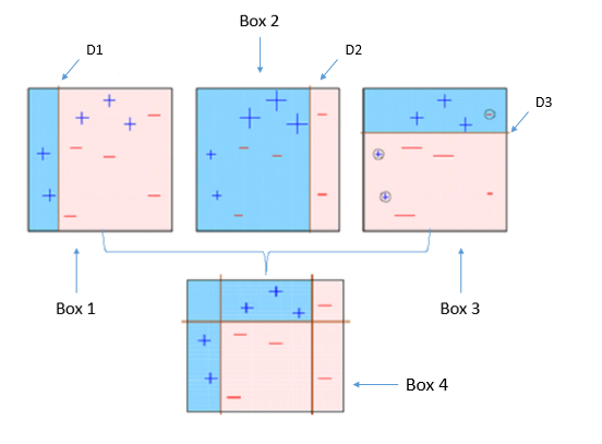
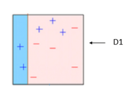
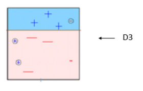
BOX – 1: In box 1 we have assigned equal weight to each data points and applied a decision stump to classify them as  + (plus) or – (minus). The decision stump (D1) has generated vertical line at left side to classify the data points. As we can see in the box vertical line has incorrectly predicted three + (plus) as – (minus). In this case, we will assign higher weights to these three + (plus) and apply another decision stump. As you can see in below image.

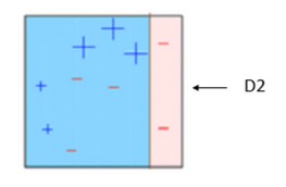
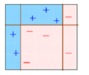
BOX – 2: Now in box 2 size of three incorrectly predicted + (plus) is bigger as compared to rest of the data points. In this case, the second decision stump (D2) will try to predict them correctly. Now, a vertical line (D2) at right side of this box has classified three mis-classified + (plus) correctly. But in this process, it has caused mis-classification errors again. This time with three -(minus). So we will assign higher weight to three – (minus) and apply another decision stump. As you can see in below image.

BOX – 3: In box 3 there are three – (minus) has been given higher weights. A decision stump (D3) is applied to predict these mis-classified observation correctly. This time a horizontal line is generated to classify + (plus) and – (minus) based on higher weight of mis-classified observation.

BOX – 4: in box 4 we will combine D1, D2 and D3 to form a strong prediction having complex rule as compared to individual weak learner. As we can see this algorithm has classified these observation quite well as compared to any of individual weak learner.

Python Code

from sklearn.ensamble import AdaBoostClassifier
clf = AdaBoostClassifier(n_estimators=4, random_state=0, algorithm=’SAMME’)
clf.fit(X, Y)

• n_estimators : integer, optional (default=50)

The maximum number of estimators at which boosting is terminated. In case of perfect fit, the learning procedure is stopped early.

• random_state : int, RandomState instance or None, optional (default=None)
• algorithm : {‘SAMME’, ‘SAMME.R’}, optional (default=’SAMME.R’)

If ‘SAMME.R’ then use the SAMME.R real boosting algorithm. base estimator must support calculation of class probabilities. If ‘SAMME’ then use the SAMME discrete boosting algorithm.

Support Vector Machine or SVM is one of the most popular Supervised Learning algorithms, which is used for Classification as well as Regression problems. However, primarily, it is used for Classification problems in Machine Learning.

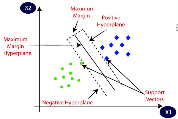
The goal of the SVM algorithm is to create the best line or decision boundary that can segregate n-dimensional space into classes so that we can easily put the new data point in the correct category in the future. This best decision boundary is called a hyperplane.

SVM chooses the extreme points/vectors that help in creating the hyperplane. These extreme cases are called as support vectors, and hence algorithm is termed as Support Vector Machine. Consider the below diagram in which there are two different categories that are classified using a decision boundary or hyperplane:

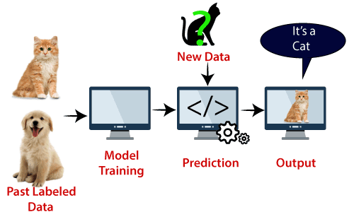
Let’s understand SVM through an example.

Suppose we see a strange cat that also has some features of dogs, so if we want a model that can accurately identify whether it is a cat or dog, so such a model can be created by using the SVM algorithm. We will first train our model with lots of images of cats and dogs so that it can learn about different features of cats and dogs, and then we test it with this strange creature. So as support vector creates a decision boundary between these two data (cat and dog) and choose extreme cases (support vectors), it will see the extreme case of cat and dog. On the basis of the support vectors, it will classify it as a cat. Consider the below diagram:

SVM algorithm can be used for Face detection, image classification, text categorization, etc.

Types of SVM:

SVM can be of two types:

• Linear SVM: Linear SVM is used for linearly separable data, which means if a dataset can be classified into two classes by using a single straight line, then such data is termed as linearly separable data, and classifier is used called as Linear SVM classifier.
• Non-linear SVM: Non-Linear SVM is used for non-linearly separated data, which means if a dataset cannot be classified by using a straight line, then such data is termed as non-linear data and classifier used is called as Non-linear SVM classifier.

Hyperplane and Support Vectors in the SVM algorithm:

Hyperplane: There can be multiple lines/decision boundaries to segregate the classes in n-dimensional space, but we need to find out the best decision boundary that helps to classify the data points. This best boundary is known as the hyperplane of SVM.

The dimensions of the hyperplane depend on the features present in the dataset, which means if there are 2 features (as shown in image), then hyperplane will be a straight line. And if there are 3 features, then hyperplane will be a 2-dimension plane.

We always create a hyperplane that has a maximum margin, which means the maximum distance between the data points.

How does SVM works?

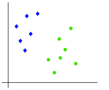
Linear SVM:

The working of the SVM algorithm can be understood by using an example. Suppose we have a dataset that has two tags (green and blue), and the dataset has two features x1 and x2. We want a classifier that can classify the pair(x1, x2) of coordinates in either green or blue. Consider the below image:

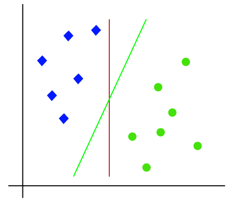
So as it is 2-d space so by just using a straight line, we can easily separate these two classes. But there can be multiple lines that can separate these classes. Consider the below image:

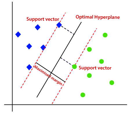
Hence, the SVM algorithm helps to find the best line or decision boundary; this best boundary or region is called as a hyperplane. SVM algorithm finds the closest point of the lines from both the classes. These points are called support vectors. The distance between the vectors and the hyperplane is called as margin. And the goal of SVM is to maximize this margin. The hyperplane with maximum margin is called the optimal hyperplane.

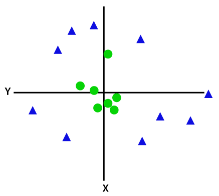
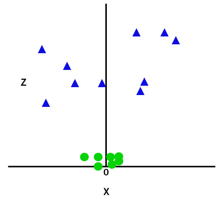
Non-Linear SVM:

If data is linearly arranged, then we can separate it by using a straight line, but for non-linear data, we cannot draw a single straight line. Consider the below image:

So to separate these data points, we need to add one more dimension. For linear data, we have used two dimensions x and y, so for non-linear data, we will add a third dimension z. It can be calculated as:

z=x2 +y2

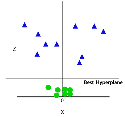
By adding the third dimension, the sample space will become as below image:

So now, SVM will divide the datasets into classes in the following way. Consider the below image:

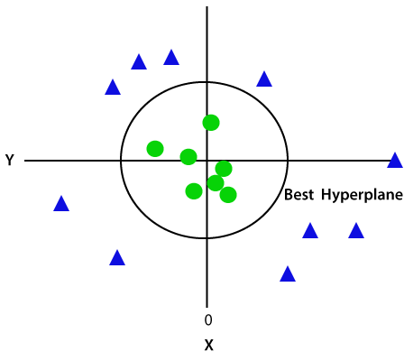
Since we are in 3-d Space, hence it is looking like a plane parallel to the x-axis. If we convert it in 2d space with z=1, then it will become as:

Hence we get a circumference of radius 1 in case of non-linear data.

We will see Python Implementation of Support Vector Machine in next chapter

Reference-

Javapoint