Archive November 2019

Matplotlib-Introduction

Matplotlib is the “grandfather” library of data visualization with Python. It was created by John Hunter. He created it to try to replicate MatLab’s (another programming language) plotting capabilities in Python. So if you happen to be familiar with matlab, matplotlib will feel natural to you.

It is an excellent 2D and 3D graphics library for generating scientific figures.

Some of the major Pros of Matplotlib are:

  • Generally easy to get started for simple plots
  • Support for custom labels and texts
  • Great control of every element in a figure
  • High-quality output in many formats
  • Very customizable in general

Matplotlib allows you to create reproducible figures programmatically. Let’s learn how to use it! I encourage you just to explore the official Matplotlib web page: http://matplotlib.org/

Installation of Matplotlib:

To install the latest release of matplotlib, you can use pip:

pip install matplotlib

You can also use conda to install the latest version of matplotlib:

conda install matplotlib

Now from next lecture we will learn how to plot different kind of charts and plot with the help of matplotlib.

Seaborn-Introduction

As per Seaborn’s official website, they state,

“If matplotlib “tries to make easy things easy and hard things possible”, seaborn tries to make a well-defined set of hard things easy too”

So we can say seaborn is an amazing python data visualization library built on top of the matplotlib.

Why one should you Seaborn instead of matplotlib?

  • Seaborn comes with a large number of high-level interfaces and customized themes where matplotlib lacks as it’s not easy to figure out the settings that makes plots attractive.
  • Matplotlib functions don’t work well with dataframes, whereas seaborn does.

Installation:

To install the latest release of seaborn, you can use pip.

pip install seaborn

You can also use conda to install the latest version of seaborn

conda install seaborn

Seaborn- Matrix Plot

Matrix plots allow you to plot data as color-encoded matrices and can also be used to indicate clusters within the data (later in the machine learning section we will learn how to formally cluster data).

So in this article we will deal with basically two plots as per follow:

  1. Heatmaps:- A heat map (or heatmap) is a graphical representation of data where values are depicted by color. Heat maps make it easy to visualize complex data and understand it at a glance. To use a heatmap the data should be in a matrix form i.e the index name and the column name must match in some way ­so that the data that we fill inside the cells are relevant.
  2. Cluster maps:- Cluster maps uses hierarchical clustering. It performs the clustering based on the similarity of the rows and columns.

Let’s begin by exploring seaborn’s heatmap and clutermap

Banking Credit Card Spend Prediction and Identify Drivers for Spends

Business Problem:

One of the global banks would like to understand what factors driving credit card spend are. The bank want use these insights to calculate credit limit. In order to solve the problem, the bank conducted survey of 5000 customers and collected data.

The objective of this case study is to understand what’s driving the total spend (Primary Card + Secondary card). Given the factors, predict credit limit for the new applicants.

Data Availability:

  • Data for the case are available in xlsx format.
  • The data have been provided for 5000 customers.
  • Detailed data dictionary has been provided for understanding the data in the data.
  • Data is encoded in the numerical format to reduce the size of the data however some of the variables are categorical. You can find the details in the data dictionary

Let’s develop a machine learning model for further analysis.

Store Sales Prediction – Forecasting

Business Context:

The objective is predicting store sales using historical markdown data. One challenge of modelling retail data is the need to make decisions based on limited history. If Christmas comes but once a year, so does the chance to see how strategic decisions impacted the bottom line.

Business Problem:

Company provided with historical sales data for 45 Walmart stores located in different regions. Each store contains a number of departments, and you are tasked with predicting the department-wide sales for each store.

In addition, Walmart runs several promotional markdown events throughout the year. These markdowns precede prominent holidays, the four largest of which are the Super Bowl, Labour Day, Thanksgiving, and Christmas. The weeks including these holidays are weighted five times higher in the evaluation than non-holiday weeks. Part of the challenge presented by this competition is modelling the effects of markdowns on these holiday weeks in the absence of complete/ideal historical data.

Data Availability:

stores.csv: This file contains anonymized information about the 45 stores, indicating the type and size of store.

train.csv: This is the historical training data, which covers to 2010-02-05 to 2012-11- 01, Within this file you will find the following fields:

  • Store – the store number
  • Dept – the department number
  • Date – the week
  • Weekly_Sales – sales for the given department in the given store
  • IsHoliday – whether the week is a special holiday week

test.csv: This file is identical to train.csv, except we have withheld the weekly sales. You must predict the sales for each triplet of store, department, and date in this file.

features.csv: This file contains additional data related to the store, department, and regional activity for the given dates. It contains the following fields:

  • Store – the store number
  • Date – the week
  • Temperature – average temperature in the region
  • Fuel_Price – cost of fuel in the region
  • MarkDown1-5 – anonymized data related to promotional markdowns that Walmart is running. MarkDown data is only available after Nov 2011, and is not available for all stores all the time. Any missing value is marked with an NA.
  • CPI – the consumer price index
  • Unemployment – the unemployment rate
  • IsHoliday – whether the week is a special holiday week

Let’s develop a machine learning model for further analysis.
Credit Card Segmentation

Data Available:

  • CC GENERAL.csv

Business Context:

A Bank wants to develop a customer segmentation to define marketing strategy. The sample dataset summarizes the usage behaviour of about 9000 active credit card holders during the last 6 months. The file is at a customer level with 18 behavioural variables.

Business Requirements:

Advanced data preparation: Build an enriched customer profile by deriving “intelligent” KPIs such as:

  • Monthly average purchase and cash advance amount
  • Purchases by type (one-off, instalments)
  • Average amount per purchase and cash advance transaction,
  • Limit usage (balance to credit limit ratio),
  • Payments to minimum payments ratio etc.
  • Advanced reporting: Use the derived KPIs to gain insight on the customer profiles.
  • Identification of the relationships/ affinities between services.
  • Clustering: Apply a data reduction technique factor analysis for variable reduction technique and a clustering algorithm to reveal the behavioural segments of credit card holders
  • Identify cluster characteristics of the cluster using detailed profiling.
  • Provide the strategic insights and implementation of strategies for given set of cluster characteristics.

Data Dictionary:

  • CUST_ID: Credit card holder ID
  • BALANCE: Monthly average balance (based on daily balance averages)
  • BALANCE_FREQUENCY: Ratio of last 12 months with balance
  • PURCHASES: Total purchase amount spent during last 12 months
  • ONEOFF_PURCHASES: Total amount of one-off purchases
  • INSTALLMENTS_PURCHASES: Total amount of installment purchases
  • CASH_ADVANCE: Total cash-advance amount
  • PURCHASES_ FREQUENCY: Frequency of purchases (Percent of months with at least one purchase)
  • ONEOFF_PURCHASES_FREQUENCY: Frequency of one-off-purchases PURCHASES_INSTALLMENTS_FREQUENCY: Frequency of installment purchases
  • CASH_ADVANCE_ FREQUENCY: Cash-Advance frequency
  • AVERAGE_PURCHASE_TRX: Average amount per purchase transaction
  • CASH_ADVANCE_TRX: Average amount per cash-advance transaction
  • PURCHASES_TRX: Average amount per purchase transaction
  • CREDIT_LIMIT: Credit limit
  • PAYMENTS: Total payments (due amount paid by the customer to decrease their statement balance) in the period
  • MINIMUM_PAYMENTS: Total minimum payments due in the period.
  • PRC_FULL_PAYMEN: Percentage of months with full payment of the due statement balance
  • TENURE: Number of months as a customer

Let’s develop a machine learning model for further analysis.

Network Intrusion Detection

In this case study we need to predict anomalies and attacks in the network.

Business Problem:

The task is to build network intrusion detection system to detect anomalies and attacks in the network.

There are two problems.

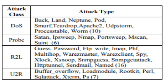
  1. Binomial Classification: Activity is normal or attack.
  2. Multinomial classification: Activity is normal or DOS or PROBE or R2L or U2R .

Data Availability:

This data is KDDCUP’99 data set, which is widely used as one of the few publicly available data sets for network-based anomaly detection systems.

For more about data you can visit to http://www.unb.ca/cic/datasets/nsl.html

BASIC FEATURES OF EACH NETWORK CONNECTION VECTOR

  1. Duration: Length of time duration of the connection
  2.  Protocol_type: Protocol used in the connection
  3.  Service: Destination network service used
  4.  Flag: Status of the connection – Normal or Error
  5.  Src_bytes: Number of data bytes transferred from source to destination in single connection
  6.  Dst_bytes: Number of data bytes transferred from destination to source in single connection
  7.  Land: if source and destination IP addresses and port numbers are equal then, this variable takes value 1 else 0
  8.  Wrong_fragment: Total number of wrong fragments in this connection
  9.  Urgent: Number of urgent packets in this connection. Urgent packets are packets with the urgent bit activated.
  10. Hot: Number of „hot‟ indicators in the content such as: entering a system directory, creating programs and executing programs.
  11. Num_failed _logins: Count of failed login attempts.
  12. Logged_in Login Status: 1 if successfully logged in; 0 otherwise.
  13. Num_compromised: Number of “compromised’ ‘ conditions.
  14. Root_shell: 1 if root shell is obtained; 0 otherwise.
  15.  Su_attempted: 1 if “su root” command attempted or used; 0 otherwise.
  16.  Num_root: Number of “root” accesses or number of operations performed as a root in the connection.
  17. Num_file_creations: Number of file creation operations in the connection.
  18. Num_shells: Number of shell prompts.
  19. Num_access_files: Number of operations on access control files .
  20. Num_outbound_cmds: Number of outbound commands in an ftp session.
  21. Is_hot_login: 1 if the login belongs to the “hot” list i.e., root or admin; else 0.
  22. Is_guest_login: 1 if the login is a “guest” login; 0 otherwise .
  23. Count: Number of connections to the same destination host as the current connection in the past two seconds
  24. Srv_count: Number of connections to the same service (port number) as the current connection in the past two seconds.
  25. Serror_rate: The percentage of connections that have activated the flag (4) s0, s1, s2 or s3, among the connections aggregated in count (23 )
  26. Srv_serror_rate: The percentage of connections that have activated the flag (4) s0, s1, s2 or s3, among the connections aggregated in srv_count (24)
  27. Rerror_rate: The percentage of connections that have activated the flag (4) REJ, among the connections aggregated in count (23)
  28. Srv_rerror_rate: The percentage of connections that have activated the flag (4) REJ, among the connections aggregated in srv_count (24)
  29. Same_srv_rate: The percentage of connections that were to the same service, among the connections aggregated in count (23)
  30. Diff_srv_rate: The percentage of connections that were to different services, among the connections aggregated in count (23)
  31. Srv_diff_host_ rate: The percentage of connections that were to different destination machines among the connections aggregated in srv_count (24)
  32. Dst_host_count: Number of connections having the same destination host IP address.
  33. Dst_host_srv_ count: Number of connections having the same port number.
  34. Dst_host_same _srv_rate: The percentage of connections that were to the same service, among the connections aggregated in dst_host_count (32) .
  35. Dst_host_diff_ srv_rate: The percentage of connections that were to different services, among the connections aggregated in dst_host_count (32)
  36. Dst_host_same _src_port_rate: The percentage of connections that were to the same source port, among the connections aggregated in dst_host_srv_c ount (33) .
  37. Dst_host_srv_ diff_host_rate: The percentage of connections that were to different destination machines, among the connections aggregated in dst_host_srv_count (33).
  38. Dst_host_serro r_rate: The percentage of connections that have activated the flag (4) s0, s1, s2 or s3, among the connections aggregated in dst_host_count (32).
  39. Dst_host_srv_s error_rate: The percent of connections that have activated the flag (4) s0, s1, s2 or s3, among the connections aggregated in dst_host_srv_c ount (33).
  40. Dst_host_rerro r_rate: The percentage of connections that have activated the flag (4) REJ, among the connections aggregated in dst_host_count (32) .
  41. Dst_host_srv_r error_rate: The percentage of connections that have activated the flag (4) REJ, among the connections aggregated in dst_host_srv_c ount (33).

Attack Class:

Let’s develop a machine learning model for further analysis.