Logistic Regression-Theory
As these days in analytics interview most of the interviewer ask questions about two algorithms which is logistic and linear regression. But why is there any reason behind?
Yes, there is a reason behind that these algorithm are very easy to interpret. I believe you should have in-depth understanding of these algorithms.
In this article we will learn about logistic regression in details. So let’s deep dive in Logistic regression.
What is Logistic Regression?
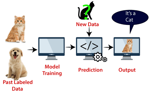
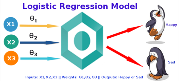
Logistic regression is a classification technique which helps to predict the probability of an outcome that can only have two values. Logistic Regression is used when the dependent variable (target) is categorical.
Types of logistic Regression:
- Binary(Pass/fail or 0/1)
- Multi(Cats, Dog, Sheep)
- Ordinal(Low, Medium, High)
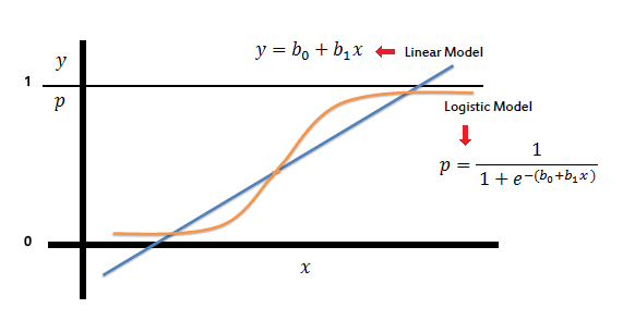
On the other hand, a logistic regression produces a logistic curve, which is limited to values between 0 and 1. Logistic regression is similar to a linear regression, but the curve is constructed using the natural logarithm of the “odds” of the target variable, rather than the probability.
What is Sigmoid Function:
To map predicted values with probabilities, we use the sigmoid function. The function maps any real value into another value between 0 and 1. In machine learning, we use sigmoid to map predictions to probabilities.
S(z) = 1/1+e−z
Where:
- s(z) = output between 0 and 1 (probability estimate)
- z = input to the function (your algorithm’s prediction e.g. b0 + b1*x)
- e = base of natural log
Graph
In Linear Regression, we use the Ordinary Least Square (OLS) method to determine the best coefficients to attain good model fit but In Logistic Regression, we use maximum likelihood method to determine the best coefficients and eventually a good model fit.
How Maximum Likelihood method works?
For a binary classification (1/0), maximum likelihood will try to find the values of b0 and b1 such that the resultant probabilities are close to either 1 or 0.
Logistic Regression Assumption:
I got a very good consolidated assumption on Towards Data science website, which I am putting here.
- Binary logistic regression requires the dependent variable to be binary.
- For a binary regression, the factor level 1 of the dependent variable should represent the desired outcome.
- Only meaningful variables should be included.
- The independent variables should be independent of each other. That is, the model should have little or no multicollinearity.
- The independent variables are linearly related to the log of odds.
- Logistic regression requires quite large sample sizes.
Performance evaluation methods of Logistic Regression.
Akaike Information Criteria (AIC):
We can say AIC works as a counter part of adjusted R square in multiple regression. The thumb rules of AIC are Smaller the better. AIC penalizes increasing number of coefficients in the model. In other words, adding more variables to the model wouldn’t let AIC increase. It helps to avoid overfitting.
To measure AIC of a single mode will not fruitful. To use AIC correctly build 2-3 logistic model and compare their AIC. The model which will have lowest AIC will relatively batter.
Null Deviance and Residual Deviance:
- Null deviance is calculated from the model with no features, i.e. only intercept. The null model predicts class via a constant probability.
- Residual deviance is calculated from the model having all the features. In both null and residual lower the value batter the model is.
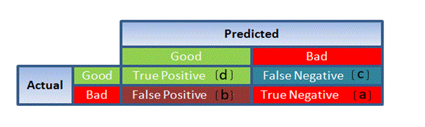
Confusion Matrix:
It is nothing but a tabular representation of Actual vs Predicted values. This helps us to find the accuracy of the model and avoid overfitting. This is how it looks like
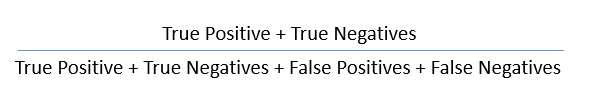
So now we can calculate the accuracy.
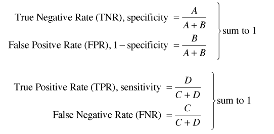
True Positive Rate (TPR):
It shows how many positive values, out of all the positive values, have been correctly predicted.
The formula to calculate the true positive rate is (TP/TP + FN). Or TPR = 1 - False Negative Rate. It is also known as Sensitivity or Recall.
False Positive Rate (FPR):
It shows how many negative values, out of all the negative values, have been incorrectly predicted.
The formula to calculate the false positive rate is (FP/FP + TN). Also, FPR = 1 - True Negative Rate.
True Negative Rate (TNR):
It represents how many negative values, out of all the negative values, have been correctly predicted. The formula to calculate the true negative rate is (TN/TN + FP). It is also known as Specificity.
False Negative Rate (FNR):
It indicates how many positive values, out of all the positive values, have been incorrectly predicted. The formula to calculate false negative rate is (FN/FN + TP).
Precision:
It indicates how many values, out of all the predicted positive values, are actually positive. The formula is (TP / TP + FP).
F Score:
F score is the harmonic mean of precision and recall. It lies between 0 and 1. Higher the value, better the model. Formula is 2((precision*recall) / (precision + recall)).
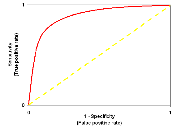
Receiver Operator Characteristic (ROC):
ROC is use to determine the accuracy of a classification model. It determines the model’s accuracy using Area Under Curve (AUC). Higher the area batter the model. ROC is plotted between True Positive Rate (Y axis) and False Positive Rate (X Axis).
In below graph yellow line represents the ROC curve at 0.5 thresholds. At this point, sensitivity = specificity.