In this project we will be working with a dummy advertising data set, indicating whether or not a particular internet user clicked on an Advertisement on a company website.
We will try to create a model that will predict whether or not they will click on an ad based off the features of that user.
This data set contains the following features:
‘Daily Time Spent on Site’: consumer time on site in minutes
‘Age’: customer age in years
‘Area Income’: Avg. Income of geographical area of consumer
‘Daily Internet Usage’: Avg. minutes a day consumer is on the internet
‘Ad Topic Line’: Headline of the advertisement
‘City’: City of consumer
‘Male’: Whether or not consumer was male
‘Country’: Country of consumer
‘Timestamp’: Time at which consumer clicked on Ad or closed window
‘Clicked on Ad’: 0 or 1 indicated clicking on Ad
Find following jupyter notebook code for detailed solution.
Decision tree is very simple yet a powerful
algorithm for classification and regression.
As name suggest it has tree like structure. It is a non-parametric technique. A
decision tree typically starts with a single node, which branches into possible
outcomes. Each of those outcomes leads to additional nodes, which branch off
into other possibilities. This gives it a treelike shape.
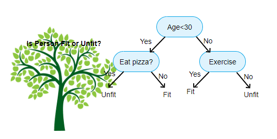
For example of a decision tree can be explained using below binary tree. Let’s suppose you want to predict whether a person is fit by their given information like age, eating habit, and physical activity, etc. The decision nodes here are questions like ‘What’s the age?’, ‘Does he exercise?’, ‘Does he eat a lot of pizzas’? And the leaves, which are outcomes like either ‘fit’, or ‘unfit’. In this case this was a binary classification problem (yes or no type problem).
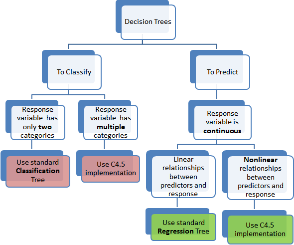
There are two main types of Decision Trees:
Classification trees (Yes/No types)
What we’ve seen above is an example of classification tree, where the outcome was a variable like ‘fit’ or ‘unfit’. Here the decision variable is categorical.
Regression trees (Continuous data types)
Here the decision or the outcome variable is Continuous, e.g. a number like 123.
Image source google.com
The top-most item, in this example, “Age < 30 ?” is called the root. It’s where everything starts from. Branches are what we call each line. A leaf is everything that isn’t the root or a branch.
A general algorithm for a decision tree can be described as follows:
Pick
the best attribute/feature. The best attribute is one which best splits or
separates the data.
Ask
the relevant question.
Follow
the answer path.
Go
to step 1 until you arrive to the answer.
Terms
used with Decision Trees:
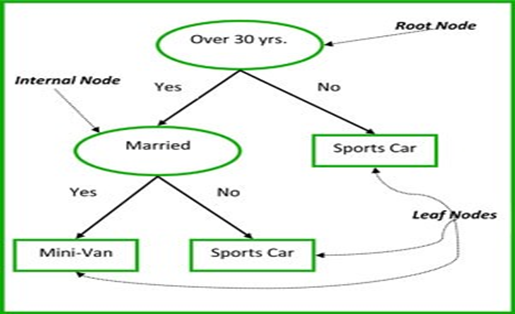
Root
Node – It represents entire population or sample and this
further gets divided into two or more similar sets.
Splitting
– Process
to divide a node into two or more sub nodes.
Decision Node – A
sub node is divided further sub node, called decision node.
Leaf/Terminal Node –
Node which do not split further called leaf node.
Pruning –
When we remove sub-nodes of a decision node, this process is called pruning.
Branch/ Sub-tree –
A sub-section of entire tree is called branch or subtree.
Parent and child node –
A node, which is divided into sub-nodes is called parent node of sub-nodes
whereas sub-nodes are the child of parent node.
Let’s understand above terms with the below image
Image Source google.com
Types of Decision Trees
Categorical Variable decision tree – Decision Tree which has categorical target variable then it called as categorical variable.
Continuous Variable Decision Tree – Decision Tree which has continuous target variable then it is called as Continuous Variable Decision Tree.
Advantages of Decision Tree
Easy to understand – Algorithm is very easy to understand even for people from non-analytical background. A person without statistical knowledge can interpret them.
Useful in data exploration – It is the fastest algorithm to identify most significant variables and relation between variables. It help us to identify those variables which has better power to predict target variable.
Decision tree do not required more effort from user side for data preparation.
This algorithm is not affected by outliers or missing value to an extent, so it required less data cleaning effort as compare to other model.
This model can handle both numerical and categorical variables.
The number of hyper-parameters to be tuned is almost null.
Disadvantages of Decision Tree
Over Fitting – It is the most common problem in decision tree. This issue has resolved by setting constraints on model parameters and pruning. Over fitting is an phenomena where your model create a complex tree that do not generalize the data very well.
Small variations in the data can
result completely different tree which mean it unstable the model. This problem
is called variance, which need to lower by method like bagging and boosting.
If some class is dominate in your
model then decision tree learner can create a biased tree. So it is recommended
to balance the data set prior to fitting with the decision tree.
Calculations can become complex
when there are many class label.
Decision Tree Flowchart
Image Source google.com
How does a tree decide where to split?
In decision tree making splits effect the accuracy of model. The decision criteria are different for classification and regression trees. Decision tree splits the nodes on all available variables and then selects the split which results in most homogeneous sub-nodes.
The algorithm
selection is also based on type of target variables. The four most commonly
used algorithms in decision tree are:
CHAID – Chi-Square Interaction Detector
CART – Classification and regression trees.
Let’s discuss both methods in detail
CHAID – Chi-Square Interaction Detector
It is an algorithm to find out the statistical significance between the differences between sub-nodes and parent node. It works with categorical target variable such as “yes” or “no”.
Algorithm follows following steps:
Iterate all available x variables.
Check if the variable is numeric
If the variable is numeric make it categorical by decile and percentile.
Figure out all possible cuts.
For each possible cut it will do Chi-Square test and store the P value
Choose that cut which give least p value.
Cut the data using that variable and that cut which gives least P value.
CART – Classification and regression trees
There are basically two subtypes for this algorithm.
Gini index:
It says, if we select two items from a population at random then they must be of same class and probability for this is 1 if population is pure. It works with categorical target variable “Success” or “Failure”.
Gini = 1-P^2 – (1-p)^2 , Here p is the probability
Gain = Gini of parents leaf – weighted average of Gini of the nodes (Weights are proportional to population of each child node)
Steps to Calculate Gini for a split
Iterate all available x variables.
Check if the variable is numeric
If the variable is numeric make it categorical by decile and percentile.
Figure out all possible cuts.
Calculate gain for each split
Choose that cut which gives the highest cut.
Cut the data using that variable and that cut which gives maximum gain
Entropy Tree:
To understand entropy tree we need to first understand what entropy is?
Entropy – Entropy is basically measures the level of impurity in a group of examples. If the sample is completely homogeneous, then the entropy is zero and if the sample is an equally divided (50% — 50%), it has entropy of one.
Entropy = -p log2 p — q log2q
Here p and q is the probability of success and failure respectively in that node. Entropy is also used with categorical target variable. It chooses the split which has lowest entropy compared to parent node and other splits. The lesser the entropy, the better it is.
Gain = Entropy of parents leaf – weighted average of entropy of the nodes (Weights are proportional to population of each child node)
Steps to Calculate Entropy for a split
Iterate all available x variables.
Check if the variable is numeric
If the variable is numeric make it categorical by decile and percentile.
Figure out all possible cuts.
Calculate gain for each split
Choose that cut which gives the highest cut.
Cut the data using that variable and that cut which gives maximum gain.
Decision Tree Regression
As we have discussed above with the help of decision tree we can also solve the regression problem. So let’s see what the steps are.
Following steps are involved in algorithm.
Iterate all available x variables.
Check if the variable is numeric
If the variable is numeric make it categorical by decile and percentile.
Figure out all possible cuts.
For each cuts calculate MSE
Choose that cut and that variable which gives the minimum MSE.
Cut the data using that variable and that cut which gives minimum MSE.
Stopping Criteria of Decision Tree
Pure
Node – If tree find a pure node, that particular leaf will stop growing.
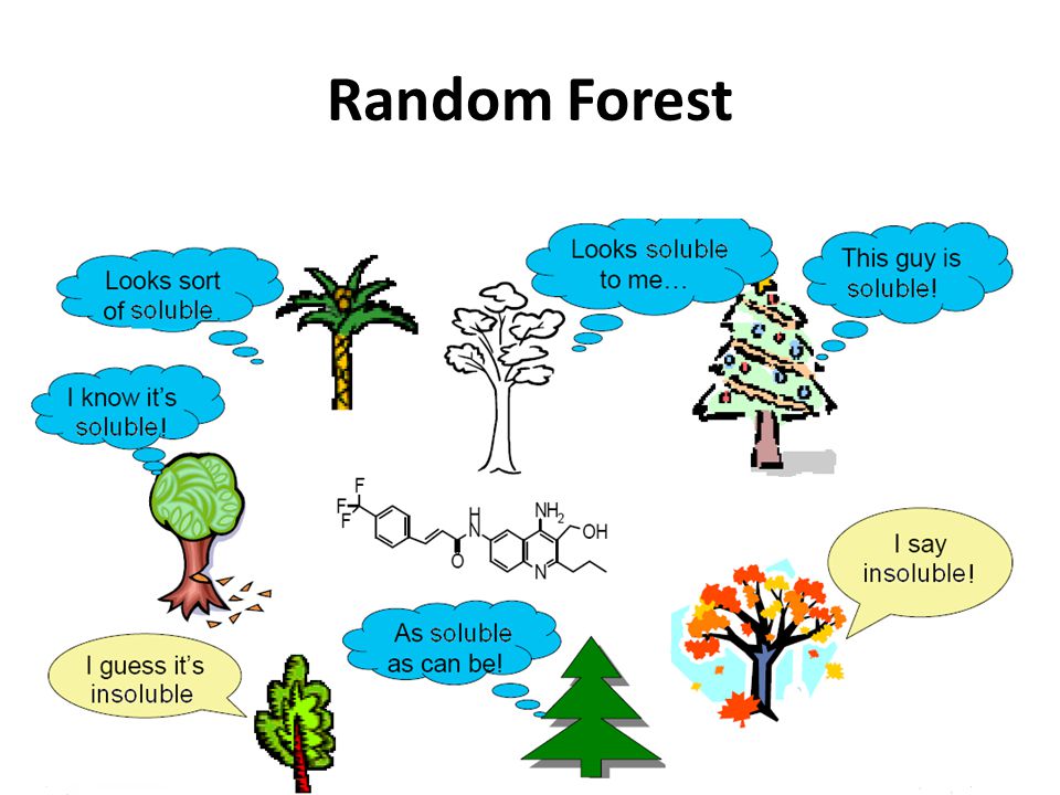
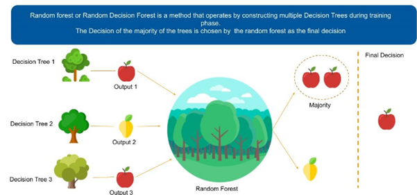
Random forest algorithm is a supervised algorithm. As you can guess from its name this algorithm creates a forest with number of trees. It operates by constructing multiple decision trees. The final decision is made based on the majority of the trees and is chosen by the random forest.
image source – google.com
The method of combining trees is known as an ensemble method. Ensembling is nothing but a combination of weak learners (individual trees) to produce a strong learner.
Let’s understand ensemble with an example. Let’s suppose you want to watch movie but you have doubt in your mind regarding it’s reviews, so you have asked 10 people who have watched the movie, 8 of them said movie is fantastic and 2 of them said movie was not good. Since the majority is in favour, you decide to watch the movie. This is how we use ensemble techniques in our daily life too.
Random Forest can be used to solve regression and classification problems. In regression problems, the dependent variable is continuous. In classification problems, the dependent variable is categorical.
Advantages and Disadvantages of Random Forest
Advantages are as follows:
It is used to solve both regression and classification problems.
It can be also used to solve unsupervised ML problems.
It can handle thousands of input variables without variable selection.
It can be used as a feature selection tool using its variable importance plot.
It takes care of missing data internally in an effective manner.
Disadvantages are as follows:
This is a black-box model so Random Forest model is difficult to interpret.
It can take longer than expected time to computer a large number of trees.
How Random Forest works?
Algorithm
can be divided into two stages.
Random forest creation.
Perform prediction from the created random forest classifier.
Random forest creation:
To create random forest we need to select following steps
Randomly select “k” features from
total “m” features, where k << m.
Among the “k” features, calculate
the node “d” using the best split point.
Split the node into child nodes using
the best split.
Repeat 1 to 3 steps until “L” number of nodes has been reached.
Build forest by repeating steps 1 to 4 for
“n” number times to create “n”
number of trees.
Perform prediction from the created random forest classifier
To perform prediction we need to take following steps
Takes the test features and use the rules of each randomly created decision tree to predict the outcomes and stores the predicted outcome (target)
Calculate the votes for each predicted target.
Consider the high voted predicted target as the final prediction from the random forest algorithm.
The minimum number of samples required to split an internal node:
If int, then consider min_samples_split as the minimum number.
If float, then min_samples_split is a percentage and ceil(min_samples_split * n_samples) are the minimum number of samples for each split.
max_features : int, float, string or None, optional (default=”auto”):
The number of features to consider when looking for the best split:
If int, then consider max_features features at each split. -If float, then max_features is a percentage and int(max_features * n_features) features are considered at each split.
If “auto”, then max_features=sqrt(n_features).
If “sqrt”, then max_features=sqrt(n_features) (same as “auto”).
If “log2”, then max_features=log2(n_features).
If None, then max_features=n_features.
max_depth : integer or None, optional (default=None):
The maximum depth of the tree. If None, then nodes are expanded until all leaves are pure or until all leaves contain less than min_samples_split samples.
max_leaf_nodes : int or None, optional (default=None):
Grow trees with max_leaf_nodes in best-first fashion. Best nodes are defined as relative reduction in impurity. If None then unlimited number of leaf nodes.
If you want to learn more about the rest of hyperparameters , check here
Support Vector Machine
or SVM is one of the most popular Supervised Learning algorithms, which is used
for Classification as well as Regression problems. However, primarily, it is
used for Classification problems in Machine Learning.
The goal of the SVM
algorithm is to create the best line or decision boundary that can segregate
n-dimensional space into classes so that we can easily put the new data point
in the correct category in the future. This best decision boundary is called a hyperplane.
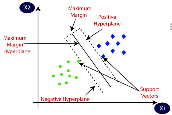
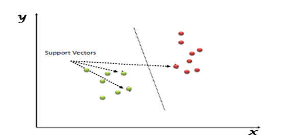
SVM chooses the extreme points/vectors that help in creating the hyperplane. These extreme cases are called as support vectors, and hence algorithm is termed as Support Vector Machine. Consider the below diagram in which there are two different categories that are classified using a decision boundary or hyperplane:
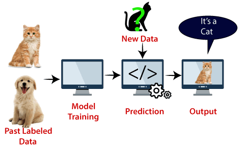
Let’s understand SVM through an example.
Suppose we see a strange cat that also has some features of dogs, so if we want a model that can accurately identify whether it is a cat or dog, so such a model can be created by using the SVM algorithm. We will first train our model with lots of images of cats and dogs so that it can learn about different features of cats and dogs, and then we test it with this strange creature. So as support vector creates a decision boundary between these two data (cat and dog) and choose extreme cases (support vectors), it will see the extreme case of cat and dog. On the basis of the support vectors, it will classify it as a cat. Consider the below diagram:
SVM algorithm can be used for Face detection, image classification, text categorization, etc.
Types of SVM:
SVM can be of two types:
Linear SVM: Linear SVM is used for linearly
separable data, which means if a dataset can be classified into two classes by
using a single straight line, then such data is termed as linearly separable
data, and classifier is used called as Linear SVM classifier.
Non-linear SVM: Non-Linear SVM is used for
non-linearly separated data, which means if a dataset cannot be classified by
using a straight line, then such data is termed as non-linear data and
classifier used is called as Non-linear SVM classifier.
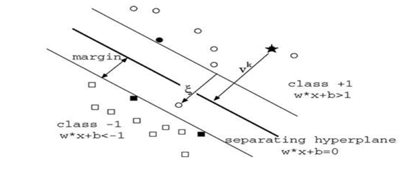
Hyperplane and Support Vectors in the SVM algorithm:
Hyperplane: There can be multiple lines/decision boundaries to segregate the classes in n-dimensional space, but we need to find out the best decision boundary that helps to classify the data points. This best boundary is known as the hyperplane of SVM.
The dimensions of the hyperplane depend on the
features present in the dataset, which means if there are 2 features (as shown
in image), then hyperplane will be a straight line. And if there are 3
features, then hyperplane will be a 2-dimension plane.
We always create a hyperplane that has a maximum margin, which means the maximum distance between the data points.
How does SVM works?
Linear SVM:
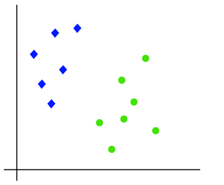
The working of the SVM algorithm can be understood
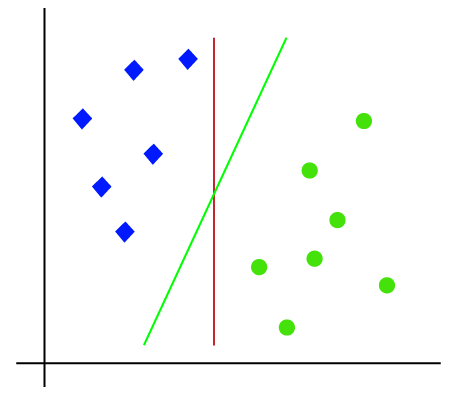
by using an example. Suppose we have a dataset that has two tags (green and
blue), and the dataset has two features x1 and x2. We want a classifier that
can classify the pair(x1, x2) of coordinates in either green or blue. Consider
the below image:
So as it is 2-d space so by just using a straight line, we can easily separate these two classes. But there can be multiple lines that can separate these classes. Consider the below image:
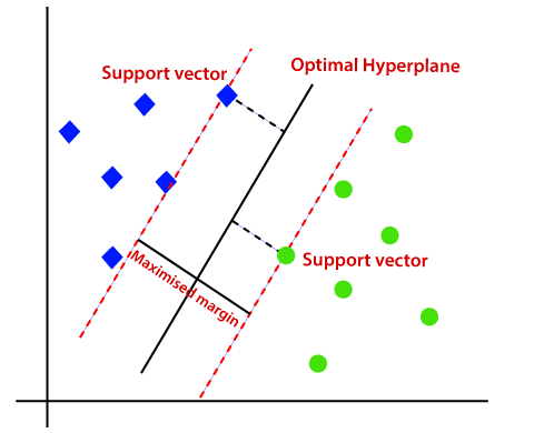
Hence, the SVM algorithm helps to find the best line or decision boundary; this best boundary or region is called as a hyperplane. SVM algorithm finds the closest point of the lines from both the classes. These points are called support vectors. The distance between the vectors and the hyperplane is called as margin. And the goal of SVM is to maximize this margin. The hyperplane with maximum margin is called the optimal hyperplane.
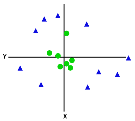
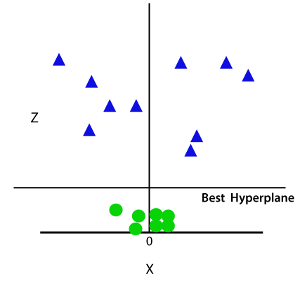
Non-Linear SVM:
If data is linearly arranged, then we can separate it by using a straight line, but for non-linear data, we cannot draw a single straight line. Consider the below image:
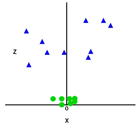
So to separate these data points, we need to add one more dimension. For linear data, we have used two dimensions x and y, so for non-linear data, we will add a third dimension z. It can be calculated as:
z=x2 +y2
By adding the third dimension, the sample space will become as below image:
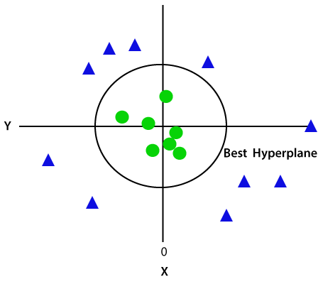
So now, SVM will divide the datasets into classes in the following way. Consider the below image:
Since we are in 3-d Space, hence it is looking like a plane parallel to the x-axis. If we convert it in 2d space with z=1, then it will become as:
Hence we get a
circumference of radius 1 in case of non-linear data.
We will see Python Implementation of Support Vector Machine in next chapter
Data Science is a combination of algorithms, tools, and machine learning technique which helps you to find common hidden patterns from the given raw data.
2. What are the differences between supervised and unsupervised learning?
Supervised Learning
Unsupervised Learning
Uses known and labeled data as input
Uses unlabeled data as input
Supervised learning has a feedback mechanism
Unsupervised learning has no feedback mechanism
The most commonly used supervised learning algorithms are decision trees, logistic regression, and support vector machine
The most commonly used unsupervised learning algorithms are k-means clustering, hierarchical clustering, and apriori algorithm
3. What do you understand by linear regression?
Linear regression helps in understanding the linear relationship between the dependent and the independent variables. Linear regression is a supervised learning algorithm, which helps in finding the linear relationship between two variables. One is the predictor or the independent variable and the other is the response or the dependent variable. In Linear Regression, we try to understand how the dependent variable changes w.r.t the independent variable. If there is only one independent variable, then it is called simple linear regression, and if there is more than one independent variable then it is known as multiple linear regression.
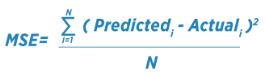
4. How do you find RMSE and MSE in a linear regression model?
RMSE and MSE are two of the most common measures of accuracy for a linear regression model. RMSE indicates the Root Mean Square Error.
MSE indicates the Mean Square Error.
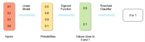
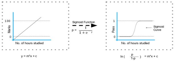
5. How is logistic regression done?
Logistic regression measures the relationship between the dependent variable (our label of what we want to predict) and one or more independent variables (our features) by estimating probability using its underlying logistic function (sigmoid).
The image shown below depicts how logistic regression works:
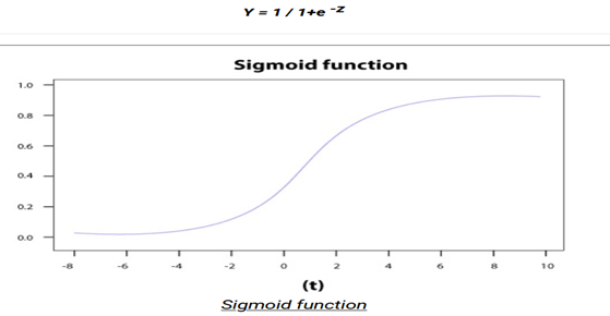
The formula and graph for the sigmoid function are as shown:
6. What is the Sigmoid Function?
It is a mathematical function having a characteristic that can take any real value and map it to between 0 to 1 shaped like the letter “S”. The sigmoid function also called a logistic function.
So, if the value of z goes to positive infinity then the predicted value of y will become 1 and if it goes to negative infinity then the predicted value of y will become 0. And if the outcome of the sigmoid function is more than 0.5 then we classify that label as class 1 or positive class and if it is less than 0.5 then we can classify it to negative class or label as class 0.
7. Why do we use the Sigmoid Function?
Sigmoid Function acts as an activation function in machine learning which is used to add non-linearity in a machine learning model, in simple words it decides which value to pass as output and what not to pass.
8. How will you explain linear regression to a non-tech person?
Linear Regression is a statistical technique of measuring the linear relationship between the two variables. By linear relationship, we mean that an increase in a variable would lead to increase in the other variable and a decrease in one variable would lead to attenuation in the second variable as well. Based on this linear relationship, we establish a model that predicts the future outcomes based on an increase in one variable.
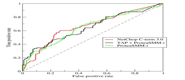
9. Explain how a ROC curve works?
The ROC curve is a graphical representation of the contrast between true positive rates and false-positive rates at various thresholds. It is often used as a proxy for the trade-off between the sensitivity (true positive rate) and false-positive rate
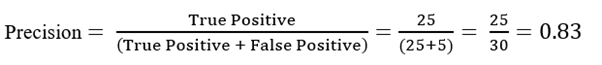
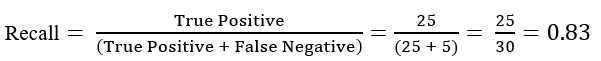
10. What is Precision, Recall, Accuracy and F1-score?
Once you have built a classification model, you need evaluate how good the predictions made by that model are. So, how do you define ‘good’ predictions?
There are some performance metrics which help us improve our models. Let us explore the differences between them for a binary classification problem:
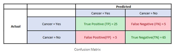
Consider the following Confusion Matrix for a classification problem which predicts whether a patient has Cancer or not for 100 patients:
Now, the following are the fundamental metrics for the above data:
Precision: It is implied as the measure of the correctly identified positive cases from all the predicted positive cases. Thus, it is useful when the costs of False Positives is high.
Recall: It is the measure of the correctly identified positive cases from all the actual positive cases. It is important when the cost of False Negatives is high.
Accuracy: One of the more obvious metrics, it is the measure of all the correctly identified cases. It is most used when all the classes are equally important.
Now for our above example, suppose that there only 30 patients who actually have cancer. What if our model identifies 25 of those as having cancer?
The accuracy in this case is = 90% which is a high enough number for the model to be considered as ‘accurate’. However, there are 5 patients who actually have cancer and the model predicted that they don’t have it. Obviously, this is too high a cost. Our model should try to minimize these False Negatives. For these cases, we use the F1-score.
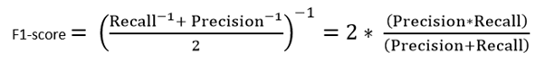
F1-score: This is the harmonic mean of Precision and Recall and gives a better measure of the incorrectly classified cases than the Accuracy Metric.
We use the Harmonic Mean since it penalizes the extreme values.
To summaries the differences between the F1-score and the accuracy,
Accuracy is used when the True Positives and True negatives are more important while F1-score is used when the False Negatives and False Positives are crucial
Accuracy can be used when the class distribution is similar while F1-score is a better metric when there are imbalanced classes as in the above case.
In most real-life classification problems, imbalanced class distribution exists and thus F1-score is a better metric to evaluate our model on.
11. How is AUC different from ROC?
AUC curve is a measurement of precision against the recall. Precision = TP/(TP + FP) and TP/(TP + FN). This is in contrast with ROC that measures and plots True Positive against False positive rate.
12. What is Selection Bias?
Selection bias is a kind of error that occurs when the researcher decides who is going to be studied. It is usually associated with research where the selection of participants isn’t random. It is sometimes referred to as the selection effect. It is the distortion of statistical analysis, resulting from the method of collecting samples. If the selection bias is not taken into account, then some conclusions of the study may not be accurate.
The types of selection bias include:
Sampling bias: It is a systematic error due to a non-random sample of a population causing some members of the population to be less likely to be included than others resulting in a biased sample.
Time interval: A trial may be terminated early at an extreme value (often for ethical reasons), but the extreme value is likely to be reached by the variable with the largest variance, even if all variables have a similar mean.
Data: When specific subsets of data are chosen to support a conclusion or rejection of bad data on arbitrary grounds, instead of according to previously stated or generally agreed criteria.
Attrition: Attrition bias is a kind of selection bias caused by attrition (loss of participants) discounting trial subjects/tests that did not run to completion
13. Differentiate between uni-variate, bi-variate, and multivariate analysis
Univariate:
Univariate data contains only one variable. The purpose of the univariate analysis is to describe the data and find patterns that exist within it.
Example: height of students.
The patterns can be studied by drawing conclusions using mean, median, mode, dispersion or range, minimum, maximum, etc.
Bivariate:
Bivariate data involves two different variables. The analysis of this type of data deals with causes and relationships and the analysis is done to determine the relationship between the two variables.
Example: temperature and ice cream sales in the summer season. Here, the relationship is visible from the table that temperature and sales are directly proportional to each other. The hotter the temperature, the better the sales.
Multivariate:
Multivariate data involves three or more variables, it is categorized under multivariate. It is similar to a bivariate but contains more than one dependent variable. Example: data for house price prediction. The patterns can be studied by drawing conclusions using mean, median, and mode, dispersion or range, minimum, maximum, etc. You can start describing the data and using it to guess what the price of the house will be.
14. Explain the steps in making a decision tree.
Following are the steps:
Step-1: Begin the tree with the root node, says S, which contains the complete dataset.
Step-2: Find the best attribute in the dataset using Attribute Selection Measure (ASM).
Step-3: Divide the S into subsets that contains possible values for the best attributes.
Step-4: Generate the decision tree node, which contains the best attribute.
Step-5: Recursively make new decision trees using the subsets of the dataset created in step -3. Continue this process until a stage is reached where you cannot further classify the nodes and called the final node as a leaf node.
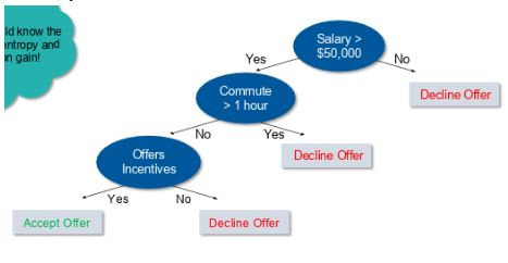
For example, let’s say you want to build a decision tree to decide whether you should accept or decline a job offer. The decision tree for this case is as shown:
It is clear from the decision tree that an offer is accepted if:
Salary is greater than $50,000
The commute is less than an hour
Incentives are offered
Attribute Selection Measures:
While implementing a Decision tree, the main issue arises that how to select the best attribute for the root node and for sub-nodes. So, to solve such problems there is a technique which is called as Attribute selection measure or ASM. By this measurement, we can easily select the best attribute for the nodes of the tree. There are two popular techniques for ASM, which are:
Information Gain
Gini Index
Information Gain:
Information gain is the measurement of changes in entropy after the segmentation of a dataset based on an attribute.
It calculates how much information a feature provides us about a class.
According to the value of information gain, we split the node and build the decision tree.
A decision tree algorithm always tries to maximize the value of information gain, and a node/attribute having the highest information gain is split first. It can be calculated using the below formula:
Information Gain= Entropy(S)- [(Weighted Avg) *Entropy(each feature)
Entropy: Entropy is a metric to measure the impurity in a given attribute. It specifies randomness in data. Entropy can be calculated as:
Entropy(s)= -P(yes)log2 P(yes)- P(no) log2 P(no)
Where,
S= Total number of samples
P(yes)= probability of yes
P(no)= probability of no
2. Gini Index:
Gini index is a measure of impurity or purity used while creating a decision tree in the CART(Classification and Regression Tree) algorithm.
An attribute with the low Gini index should be preferred as compared to the high Gini index.
It only creates binary splits, and the CART algorithm uses the Gini index to create binary splits.
Gini index can be calculated using the below formula:
Gini Index= 1- ∑jPj2
15. How do you build a random forest model?
A random forest is built up of a number of decision trees. If you split the data into different packages and make a decision tree in each of the different groups of data, the random forest brings all those trees together.
Steps to build a random forest model:
Randomly select ‘k’ features from a total of ‘m’ features where k << m
Among the ‘k’ features, calculate the node D using the best split point
Split the node into daughter nodes using the best split
Repeat steps two and three until leaf nodes are finalized
Build forest by repeating steps one to four for ‘n’ times to create ‘n’ number of trees
16. What is bias-variance trade-off?
Bias: Bias is an error introduced in your model due to oversimplification of the machine learning algorithm. It can lead to underfitting. When you train your model at that time model makes simplified assumptions to make the target function easier to understand.
Low bias machine learning algorithms — Decision Trees, k-NN and SVM High bias machine learning algorithms — Linear Regression, Logistic Regression
Variance: Variance is how much your model changes based on the changes in the input. It is an error introduced in your model due to complex machine learning algorithm, your model learns noise also from the training data set and performs badly on test data set. It can lead to high sensitivity and overfitting.
Bias-Variance trade-off: The goal of any supervised machine learning algorithm is to have low bias and low variance to achieve good prediction performance.
Example:
The k-nearest neighbour algorithm has low bias and high variance, but the trade-off can be changed by increasing the value of k which increases the number of neighbours that contribute to the prediction and in turn increases the bias of the model.
The support vector machine algorithm has low bias and high variance, but the trade-off can be changed by increasing the C parameter that influences the number of violations of the margin allowed in the training data which increases the bias but decreases the variance.
17. How can you avoid the overfitting your model?
Overfitting refers to a model that is only set for a very small amount of data and ignores the bigger picture. There are three main methods to avoid overfitting:
Keep the model simple – Take fewer variables into account, thereby removing some of the noise in the training data
Use cross-validation techniques, such as k folds cross-validation
Use regularization techniques, such as LASSO, that penalize certain model parameters if they’re likely to cause overfitting.
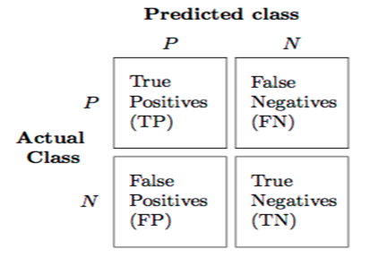
18. What is a confusion matrix?
The confusion matrix is a 2X2 table that contains 4 outputs provided by the binary classifier. Various measures, such as error-rate, accuracy, specificity, sensitivity, precision and recall are derived from it. Confusion Matrix.
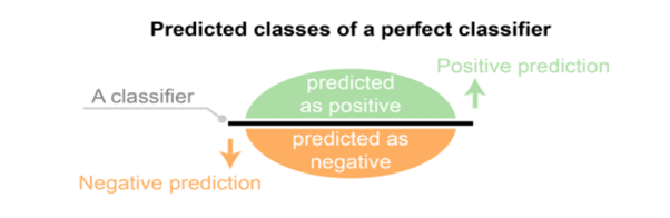
A data set used for performance evaluation is called a test data set. It should contain the correct labels and predicted labels.
The predicted labels will exactly the same if the performance of a binary classifier is perfect.
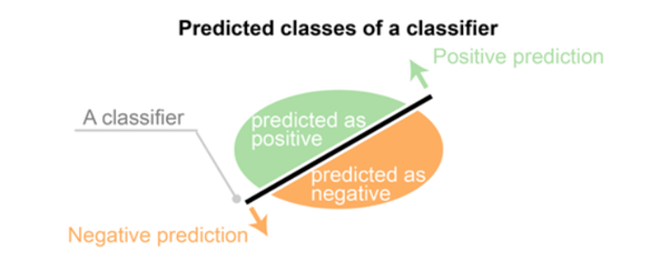
The predicted labels usually match with part of the observed labels in real-world scenarios.
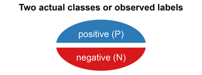
A binary classifier predicts all data instances of a test data set as either positive or negative. This produces four outcomes-
F-Score(Harmonic mean of precision and recall) = (1+b)(PREC.REC)/(b²PREC+REC) where b is commonly 0.5, 1, 2.
19. What is the difference between classification and regression?
Classification is used to produce discrete results, classification is used to classify data into some specific categories. For example, classifying emails into spam and non-spam categories.
Whereas, We use regression analysis when we are dealing with continuous data, for example predicting stock prices at a certain point in time.
20. What is meant by ‘Training set’ and ‘Test Set’?
We split the given data set into two different sections namely,’Training set’ and ‘Test Set’. ‘Training set’ is the portion of the dataset used to train the model.
‘Testing set’ is the portion of the dataset used to test the trained model.
21. How Do You Handle Missing or Corrupted Data in a Dataset?
One of the easiest ways to handle missing or corrupted data is to drop those rows or columns or replace them entirely with some other value.
There are two useful methods in Pandas:
IsNull() and dropna() will help to find the columns/rows with missing data and drop them
Fillna() will replace the wrong values with a placeholder value
22. What are the feature selection methods used to select the right variables?
Following are the technique to select features:
Principle component analysis(PCA)
t-Sne
Random forest
Forward Selection: We test one feature at a time and keep adding them until we get a good fit.
Backward Selection: We test all the features and start removing them to see what works better
23.You are given a data set consisting of variables with more than 30 percent missing values. How will you deal with them?
The following are ways to handle missing data values:
If the data set is large, we can just simply remove the rows with missing data values. It is the quickest way; we use the rest of the data to predict the values.
For smaller data sets, we can substitute missing values with the mean or average of the rest of the data using the pandas’ data frame in python. There are different ways to do so, such as df.mean(), df.fillna(mean).
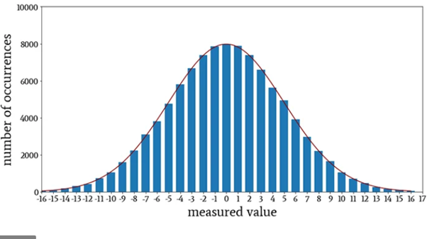
24. What do you understand by the term Normal Distribution?
Data is usually distributed in different ways with a bias to the left or to the right or it can all be jumbled up.
However, there are chances that data is distributed around a central value without any bias to the left or right and reaches normal distribution in the form of a bell-shaped curve.
The random variables are distributed in the form of a symmetrical, bell-shaped curve.
Properties of Normal Distribution are as follows;
Unimodal -one mode
Symmetrical -left and right halves are mirror images
Bell-shaped -maximum height (mode) at the mean
Mean, Mode, and Median are all located in the centre
25. What is the goal of A/B Testing?
It is a hypothesis testing for a randomized experiment with two variables A and B.
The goal of A/B Testing is to identify any changes to the web page to maximize or increase the outcome of interest. A/B testing is a fantastic method for figuring out the best online promotional and marketing strategies for your business. It can be used to test everything from website copy to sales emails to search ads
An example of this could be identifying the click-through rate for a banner ad.
26. What is p-value?
When you perform a hypothesis test in statistics, a p-value can help you determine the strength of your results. p-value is a number between 0 and 1. Based on the value it will denote the strength of the results. The claim which is on trial is called the Null Hypothesis.
Low p-value (≤ 0.05) indicates strength against the null hypothesis which means we can reject the null Hypothesis. High p-value (≥ 0.05) indicates strength for the null hypothesis which means we can accept the null Hypothesis p-value of 0.05 indicates the Hypothesis could go either way. To put it in another way, High P values: your data are likely with a true null. Low P values: your data are unlikely with a true null.
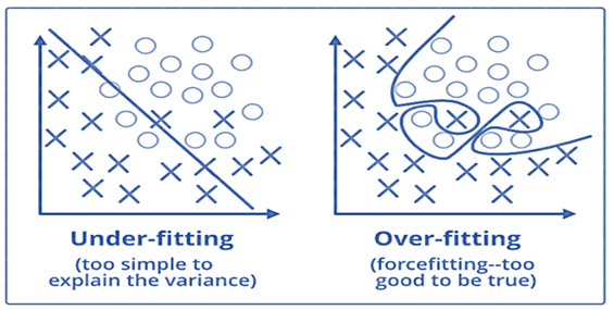
27. What are the differences between over-fitting and under-fitting?
In statistics and machine learning, one of the most common tasks is to fit a model to a set of training data, so as to be able to make reliable predictions on general untrained data.
In overfitting, a statistical model describes random error or noise instead of the underlying relationship. Overfitting occurs when a model is excessively complex, such as having too many parameters relative to the number of observations. A model that has been overfitted, has poor predictive performance, as it overreacts to minor fluctuations in the training data.
Underfitting occurs when a statistical model or machine learning algorithm cannot capture the underlying trend of the data. Underfitting would occur, for example, when fitting a linear model to non-linear data. Such a model too would have poor predictive performance.
28. How to combat Overfitting and Underfitting?
To combat overfitting and underfitting, you can resample the data to estimate the model accuracy (k-fold cross-validation) and by having a validation dataset to evaluate the model.
29. Explain cross-validation.
Cross-validation is a model validation technique for evaluating how the outcomes of a statistical analysis will generalize to an independent data set. It is mainly used in backgrounds where the objective is to forecast and one wants to estimate how accurately a model will accomplish in practice.
The goal of cross-validation is to term a data set to test the model in the training phase (i.e. validation data set) to limit problems like overfitting and gain insight into how the model will generalize to an independent data set.
30. What is k-fold cross-validation?
In k-fold cross-validation, we divide the dataset into k equal parts. After this, we loop over the entire dataset k times. In each iteration of the loop, one of the k parts is used for testing, and the other k − 1 parts are used for training. Using k-fold cross-validation, each one of the k parts of the dataset ends up being used for training and testing purposes.
31. How should you maintain a deployed model?
The steps to maintain a deployed model are:
Monitor:
Constant monitoring of all models is needed to determine their performance accuracy. When you change something, you want to figure out how your changes are going to affect things. This needs to be monitored to ensure it’s doing what it’s supposed to do.
Evaluate:
Evaluation metrics of the current model are calculated to determine if a new algorithm is needed.
Compare:
The new models are compared to each other to determine which model performs the best.
Rebuild:
The best performing model is re-built on the current state of data.
32. What is ‘Naive’ in a Naive Bayes?
The Naive Bayes Algorithm is based on the Bayes Theorem. Bayes’ theorem describes the probability of an event, based on prior knowledge of conditions that might be related to the event.
The Algorithm is ‘naive’ because it makes assumptions that may or may not turn out to be correct.
33. Explain SVM algorithm in detail.
SVM stands for support vector machine, it is a supervised machine learning algorithm which can be used for both Regression and Classification. If you have n features in your training data set, SVM tries to plot it in n-dimensional space with the value of each feature being the value of a particular coordinate. SVM uses hyperplanes to separate out different classes based on the provided kernel function.
34. What are the support vectors in SVM?
In the diagram, we see that the thinner lines mark the distance from the classifier to the closest data points called the support vectors (darkened data points). The distance between the two thin lines is called the margin.
35. What are the different kernels in SVM?
There are four types of kernels in SVM:
Linear Kernel
Polynomial kernel
Radial basis kernel
Sigmoid kernel
36. What is pruning in Decision Tree?
As the name implies, pruning involves cutting back the tree. Pruning is one of the techniques that is used to overcome our problem of Overfitting.
Pruning, in its literal sense, is a practice which involves the selective removal of certain parts of a tree(or plant), such as branches, buds, or roots, to improve the tree’s structure, and promote healthy growth. This is exactly what Pruning does to our Decision Trees as well. It makes it versatile so that it can adapt if we feed any new kind of data to it, thereby fixing the problem of overfitting. It reduces the size of a Decision Tree which might slightly increase your training error but drastically decrease your testing error, hence making it more adaptable.
37. What are Recommender Systems?
Recommender Systems are a subclass of information filtering systems that are meant to predict the preferences or ratings that a user would give to a product.
Recommender systems are widely used in movies, news, research articles, products, social tags, music, etc.Examples include movie recommenders in IMDB, Netflix & BookMyShow, product recommenders in e-commerce sites like Amazon, eBay & Flipkart, YouTube video recommendations and game recommendations in Xbox
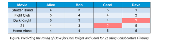
38. What is Collaborative filtering?
The process of filtering used by most of the recommender systems to find patterns or information by collaborating viewpoints, various data sources and multiple agents.
An example of collaborative filtering can be to predict the rating of a particular user based on his/her ratings for other movies and others’ ratings for all movies. This concept is widely used in recommending movies in IMDB, Netflix & BookMyShow, product recommenders in e-commerce sites like Amazon, eBay & Flipkart, YouTube video recommendations and game recommendations in Xbox
39. How will you define the number of clusters in a clustering algorithm?
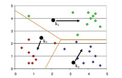
Though the Clustering Algorithm is not specified, this question is mostly in reference to K-Means clustering where “K” defines the number of clusters. The objective of clustering is to group similar entities in a way that the entities within a group are similar to each other but the groups are different from each other.
For example, the following image shows three different groups.
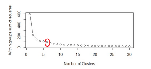
Within Sum of squares is generally used to explain the homogeneity within a cluster. If you plot WSS for a range of number of clusters, you will get the plot shown below.
The Graph is generally known as Elbow Curve.
Red circled a point in above graph i.e. Number of Cluster =6is the point after which you don’t see any decrement in WSS.
This point is known as the bending point and taken as K in K – Means.
This is the widely used approach but few data scientists also use Hierarchical clustering first to create dendrograms and identify the distinct groups from there.
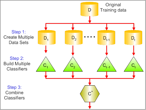
40. Describe in brief any type of Ensemble Learning?
Ensemble learning has many types but two more popular ensemble learning techniques are mentioned below.
Bagging
Bagging tries to implement similar learners on small sample populations and then takes a mean of all the predictions. In generalised bagging, you can use different learners on different population. As you expect this helps us to reduce the variance error.
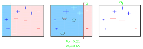
Boosting
Boosting is an iterative technique which adjusts the weight of an observation based on the last classification. If an observation was classified incorrectly, it tries to increase the weight of this observation and vice versa. Boosting in general decreases the bias error and builds strong predictive models. However, they may over fit on the training data.
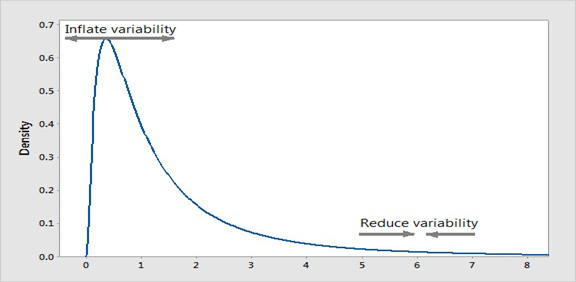
41. What is a Box-Cox Transformation?
A Box cox transformation is a statistical technique to transform non-normal dependent variables into a normal shape. If the given data is not normal then most of the statistical techniques assume normality. Applying a box cox transformation means that you can run a broader number of tests.
A Box-Cox transformation is a way to transform non-normal dependent variables into a normal shape. Normality is an important assumption for many statistical techniques, if your data isn’t normal, applying a Box-Cox means that you are able to run a broader number of tests.
42. Explain Principle Component Analysis (PCA).
PCA is a method for transforming features in a dataset by combining them into uncorrelated linear combinations.
These new features, or principal components, sequentially maximize the variance represented (i.e. the first principal component has the most variance, the second principal component has the second most, and so on).
As a result, PCA is useful for dimensionality reduction because you can set an arbitrary variance cutoff.
43. How is KNN different from k-means clustering?
K-Nearest Neighbors is a supervised classification algorithm, while k-means clustering is an unsupervised clustering algorithm. While the mechanisms may seem similar at first, what this really means is that in order for K-Nearest Neighbors to work, you need labeled data you want to classify an unlabeled point into (thus the nearest neighbor part). K-means clustering requires only a set of unlabeled points and a threshold: the algorithm will take unlabeled points and gradually learn how to cluster them into groups by computing the mean of the distance between different points.
44. You’ve built a random forest model with 10000 trees. You got delighted after getting training error as 0.00. But, the validation error is 34.23. What is going on? Haven’t you trained your model perfectly?
The model has overfitted. Training error 0.00 means the classifier has mimicked the training data patterns to an extent, that they are not available in the unseen data. Hence, when this classifier was run on an unseen sample, it couldn’t find those patterns and returned predictions with higher error. In a random forest, it happens when we use a larger number of trees than necessary. Hence, to avoid this situation, we should tune the number of trees using cross-validation.
45. In k-means or kNN, we use euclidean distance to calculate the distance between nearest neighbors. Why not manhattan distance?
We don’t use manhattan distance because it calculates distance horizontally or vertically only. It has dimension restrictions. On the other hand, the euclidean metric can be used in any space to calculate distance. Since the data points can be present in any dimension, euclidean distance is a more viable option.
Example: Think of a chessboard, the movement made by a bishop or a rook is calculated by manhattan distance because of their respective vertical & horizontal movements.
46. When does regularization becomes necessary in Machine Learning?
Regularization becomes necessary when the model begins to overfit/underfit. This technique introduces a cost term for bringing in more features with the objective function. Hence, it tries to push the coefficients for many variables to zero and hence reduce the cost term. This helps to reduce model complexity so that the model can become better at predicting (generalizing).
47. When would you use random forests Vs SVM and why?
There are a couple of reasons why a random forest is a better choice of the model than a support vector machine:
Random forests allow you to determine the feature importance. SVM’s can’t do this.
Random forests are much quicker and simpler to build than an SVM.
For multi-class classification problems, SVMs require a one-vs-rest method, which is less scalable and more memory intensive.
48. Do you think 50 small decision trees are better than a large one? Why?
Another way of asking this question is “Is a random forest a better model than a decision tree?” And the answer is yes because a random forest is an ensemble method that takes many weak decision trees to make a strong learner. Random forests are more accurate, more robust, and less prone to overfitting.
49. What’s the Relationship between True Positive Rate and Recall?
The True positive rate in machine learning is the percentage of the positives that have been properly acknowledged, and recall is just the count of the results that have been correctly identified and are relevant. Therefore, they are the same things, just having different names. It is also known as sensitivity.
50. What are Eigenvectors and Eigenvalues?
Eigenvectors are used for understanding linear transformations. In data analysis, we usually calculate the eigenvectors for a correlation or covariance matrix. Eigenvectors are the directions along which a particular linear transformation acts by flipping, compressing or stretching.
Eigenvalue can be referred to as the strength of the transformation in the direction of eigenvector or the factor by which the compression occurs.
51. What is pickle module in Python?
For serializing and de-serializing an object in Python, we make use of pickle module. In order to save this object on drive, we make use of pickle. It converts an object structure into character stream.
52. How K-means clustering works? explain in details.
The first property of clusters – it states that the points within a cluster should be similar to each other. So, our aim here is to minimize the distance between the points within a cluster.
There is an algorithm that tries to minimize the distance of the points in a cluster with their centroid – the k-means clustering technique.
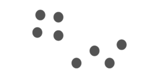
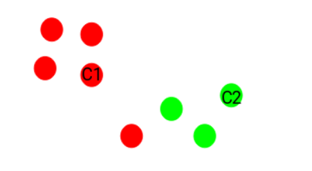
Let’s now take an example to understand how K-Means actually works:
We have these 8 points and we want to apply k-means to create clusters for these points. Here’s how we can do it.
Step 1: Choose the number of clusters k.
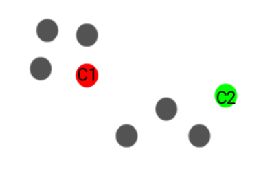
Step 2: Select k random points from the data as centroids:
Next, we randomly select the centroid for each cluster. Let’s say we want to have 2 clusters, so k is equal to 2 here. We then randomly select the centroid:
Here, the red and green circles represent the centroid for these clusters.
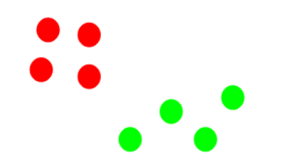
Step 3: Assign all the points to the closest cluster centroid
Once we have initialized the centroids, we assign each point to the closest cluster centroid:
Here you can see that the points which are closer to the red point are assigned to the red cluster whereas the points which are closer to the green point are assigned to the green cluster.
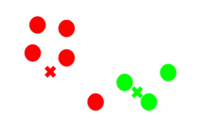
Step 4: Re-compute the centroids of newly formed clusters
Now, once we have assigned all of the points to either cluster, the next step is to compute the centroids of newly formed clusters:
Here, the red and green crosses are the new centroids.
Step 5: Repeat steps 3 and 4
We then repeat steps 3 and 4:
The step of computing the centroid and assigning all the points to the cluster based on their distance from the centroid is a single iteration. But wait – when should we stop this process? It can’t run till eternity, right?
Stopping Criteria for K-Means Clustering:
There are essentially three stopping criteria that can be adopted to stop the K-means algorithm:
Centroids of newly formed clusters do not change
Points remain in the same cluster
Maximum number of iterations are reached
53. How to test Accuracy of K-means clustering Algorithm?
To evaluate accuracy of K-Means clustering algorithm we need to do Silhouette analysis.
Silhouette analysis can be used to determine the degree of separation between clusters. For each sample:
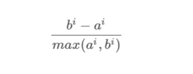
Compute the average distance from all data points in the same cluster (ai).
Compute the average distance from all data points in the closest cluster (bi).
Compute the coefficient:
The coefficient can take values in the interval [-1, 1].
If it is 0 –> the sample is very close to the neighboring clusters.
It it is 1 –> the sample is far away from the neighboring clusters.
It it is -1 –> the sample is assigned to the wrong clusters.
Therefore, we want the coefficients to be as big as possible and close to 1 to have a good clusters.
So for every K we should calculate silhouette score, and we can see the performance by graphs.
54. What are the disadvantages of K-Means clustering?
Following are the Disadvantages of K-Means Clustering:
K-Means assumes spherical shapes of clusters (with radius equal to the distance between the centroid and the furthest data point) and doesn’t work well when clusters are in different shapes such as elliptical clusters.
If there is overlapping between clusters, k-Means doesn’t have an intrinsic measure for uncertainty for the examples belong to the overlapping region in order to determine for which cluster to assign each data point.
K-Means may still cluster the data even if it can’t be clustered such as data that comes from uniform distributions.
55. What is XG Boost ?
XGboost is the most widely used algorithm in machine learning, whether the problem is a classification or a regression problem. It is known for its good performance as compared to all other machine learning algorithms.
“It is the execution of gradient boosted decision trees that is designed for high speed and performance.”
Gradient boosting is a method where the new models are created that computes the error in the previous model and then leftover is added to make the final prediction.
56. Why XG Boost is a powerful Machine leaning algorithm ?
Following are the reason behind the good performance of XGboost:
Regularization:
This is considered to be as a dominant factor of the algorithm. Regularization is a technique that is used to get rid of overfitting of the model.
Cross-Validation:
We use cross-validation by importing the function from sklearn but XGboost is enabled with inbuilt CV function.
Missing Value:
It is designed in such a way that it can handle missing values. It finds out the trends in the missing values and apprehends them.
Flexibility:
It gives the support to objective functions. They are the function used to evaluate the performance of the model and also it can handle the user-defined validation metrics.
Save and load:
It gives the power to save the data matrix and reload afterwards that saves the resources and time.