Absenteeism prediction implementation with Python Part-1
Now we will see here how to develop algorithm to predict absenteeism in python.
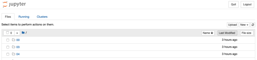
So, lets see the jupyter notebook file how I have done it.
Now we will see here how to develop algorithm to predict absenteeism in python.
So, lets see the jupyter notebook file how I have done it.
As we have already prepare the model now we need to import it in a new jupyter notebook file.
Predict the data for new data frame and store it into Mysql database. Import the library pymysql and and insert the new predicted data.
Lets see how we can do it in jupyter notebook.
One of the global banks would like to understand what factors driving credit card spend are. The bank want use these insights to calculate credit limit. In order to solve the problem, the bank conducted survey of 5000 customers and collected data.
The objective of this case study is to understand what’s driving the total spend (Primary Card + Secondary card). Given the factors, predict credit limit for the new applicants.
Let’s develop a machine learning model for further analysis.
The objective is predicting store sales using historical markdown data. One challenge of modelling retail data is the need to make decisions based on limited history. If Christmas comes but once a year, so does the chance to see how strategic decisions impacted the bottom line.
Company provided with historical sales data for 45 Walmart stores located in different regions. Each store contains a number of departments, and you are tasked with predicting the department-wide sales for each store.
In addition, Walmart runs several promotional markdown events throughout the year. These markdowns precede prominent holidays, the four largest of which are the Super Bowl, Labour Day, Thanksgiving, and Christmas. The weeks including these holidays are weighted five times higher in the evaluation than non-holiday weeks. Part of the challenge presented by this competition is modelling the effects of markdowns on these holiday weeks in the absence of complete/ideal historical data.
stores.csv: This file contains anonymized information about the 45 stores, indicating the type and size of store.
train.csv: This is the historical training data, which covers to 2010-02-05 to 2012-11- 01, Within this file you will find the following fields:
test.csv: This file is identical to train.csv, except we have withheld the weekly sales. You must predict the sales for each triplet of store, department, and date in this file.
features.csv: This file contains additional data related to the store, department, and regional activity for the given dates. It contains the following fields:
Let’s develop a machine learning model for further analysis.
A Bank wants to develop a customer segmentation to define marketing strategy. The sample dataset summarizes the usage behaviour of about 9000 active credit card holders during the last 6 months. The file is at a customer level with 18 behavioural variables.
Advanced data preparation: Build an enriched customer profile by deriving “intelligent” KPIs such as:
Let’s develop a machine learning model for further analysis.
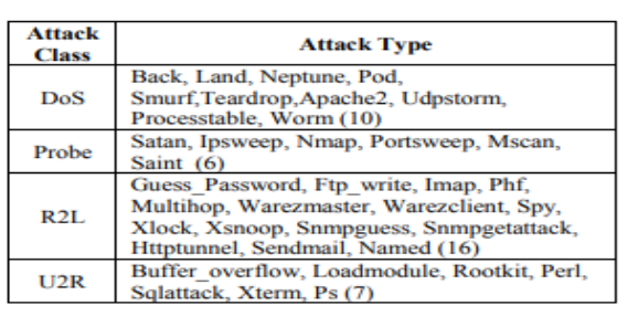
In this case study we need to predict anomalies and attacks in the network.
The task is to build network intrusion detection system to detect anomalies and attacks in the network.
There are two problems.
This data is KDDCUP’99 data set, which is widely used as one of the few publicly available data sets for network-based anomaly detection systems.
For more about data you can visit to http://www.unb.ca/cic/datasets/nsl.html
Let’s develop a machine learning model for further analysis.
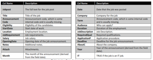
The project seeks to understand the overall demand for labour in the Armenian online job market from the 19,000 job postings from 2004 to 2015 posted on Career Center, an Armenian human resource portal. Through text mining on this data, we will be able to understand the nature of the ever-changing job market, as well as the overall demand for labour in the Armenia economy. The data was originally scraped from a Yahoo! Mailing group.
Our main business objectives are to understand the dynamics of the labour market of Armenia using the online job portal post as a proxy. A secondary objective is to implement advanced text analytics as a proof of concept to create additional features such as enhanced search function that can add additional value to the users of the job portal.
So as a Data scientist you need to answer following business questions .
Job Nature and Company Profiles:
What are the types of jobs that are in demand in Armenia? How are the job natures changing over time?
Desired Characteristics and Skill-Sets:
What are the desired characteristics and skill -set of the candidates based on the job description dataset? How these are desired characteristics changing over time?
IT Job Classification:
Build a classifier that can tell us from the job description and company description whether a job is IT or not, so that this column can be automatically populated for new job postings. After doing so, understand what important factors are which drives this classification.
Similarity of Jobs:
Given a job title, find the 5 top jobs that are of a similar nature, based on the job post.
For the IT Job classification business question, you should aim to create supervised learning classification models that are able to classify based on the job text data accurately, is it an IT job.
On the business question of Job Nature and Company Profiles. Unsupervised learning techniques, such as topic modelling and other techniques such as term frequency counting will be applied to the data, including time period segmented dataset. Qualitative assessment will be done on the results to help us understand the job postings.
To understand the desired characteristics and skill -sets demanded by employers in the job ads, unsupervised learning methods such as K-means clustering will be used after appropriate dimension reduction.
For Job Queries business question, we propose exploring the usage of Latent Semantic Model and Matrix Similarity methods for information retrieval. The results will be assessed qualitatively. To return the top 5 most similar job posting, the job text data are vectorised using different models such as word2vec, and doc2vec and similarity scores are obtained using cosine similarity scores, ranked and returned as the answer which is then evaluated individually for relevance.
The data was obtained from Kaggle competition. Each row represents a job post. The dataset representation is tabular, but many of the columns are textual/unstructured in nature. Most notably, the columns job Description, Job Requirement, Required Qual, ApplicationP and AboutC are textual. The column job post is an amalgamation of these various textual columns.
Also provided sample job posting (attached with data set)

Let’s develop a machine learning model for further analysis.
Central banks collecting information about customer satisfaction with the services provided by different bank. Also collects the information about the complaints.
So the Business Requirement is to analyze customer reviews and predict customer satisfaction with the reviews. It should include following tasks.
BankReviews.xlsx.
The data is a detailed dump of customer reviews/complaints (~500) of different services at different banks.
Let’s develop a machine learning model for further analysis.
Python is very easy to learn and implement. For many people including myself python language is easy to fall in love with. Since his first appearance in 1991, python popularity is increasing day by day. Among interpreted languages Python is distinguished by its large and active scientific computing community. Adoption of Python for scientific computing in both industry applications and academic research has increased significantly since the early 2000s.
For data analysis and exploratory analysis and data visualization, Python has upper hand as compare with the many other domain-specific open source and commercial programming languages and tools, such as R, MATLAB, SAS, Stata, and others. In recent years, Python’s improved library support (primarily pandas) has made it a strong alternative for data manipulation tasks. Combined with python’s strength in general purpose programming, it is an excellent choice as a single language for building data-centric applications.
So in short we can say due to following reason we should choose python for data analysis.
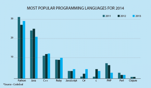
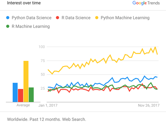
As you can see below chart, python is the most shouting language in the industry.
To successfully create and run the code we will required environment set up which will have both general-purpose python as well as the special packages required for Data science.
In this tutorial we will discuss about python 3, because Python 2 won’t be supported after 2020 and Python 3 has been around since 2008. So if you are new to Python, it is definitely worth much more to learn the new Python 3 and not the old Python 2.
Anaconda is a package manager, an environment manager, a Python/R data science distribution, and a collection of over 1,500+ open source packages. Anaconda is free and easy to install, and it offers free community support too.
To Download Anaconda click on https://www.anaconda.com/distribution/
Over 250+ packages are automatically installed with Anaconda. You can also download other packages using the pip install command.
If you need installation guide you can check the same on anaconda website https://docs.anaconda.com/anaconda/install/
From the Start menu, click the Anaconda Navigator desktop app.